Geocomputation with R - 06

The exercise solutions of Chapter 6 could be accessed at Chapter 6: Reprojecting geographic data. Here are solutions of mine explained in Chinese.

第六章 Reprojecting geographic data 详细讲述了地理数据对象的坐标参考系（coordinate reference systens, CRSs）概念，并着重讲解如何在实际应用中进行坐标参考系的转换，因为许多地理操作都需要在相同的坐标参考系之下。

解决问题

会查看地理对象的坐标参考系，会比较不同地理参考系的不同（Q1）。
会更改矢量对象的坐标参考系（使用 st_transform() 函数）（Q2）。
会更改栅格对象的坐标参考系（使用 projectRaster() 函数）（Q3&Q4）。
会根据要求定义新的投影（Q5）。

所需R包

library(sf)
library(raster)
library(dplyr)
library(spData)
library(spDataLarge)

Q1

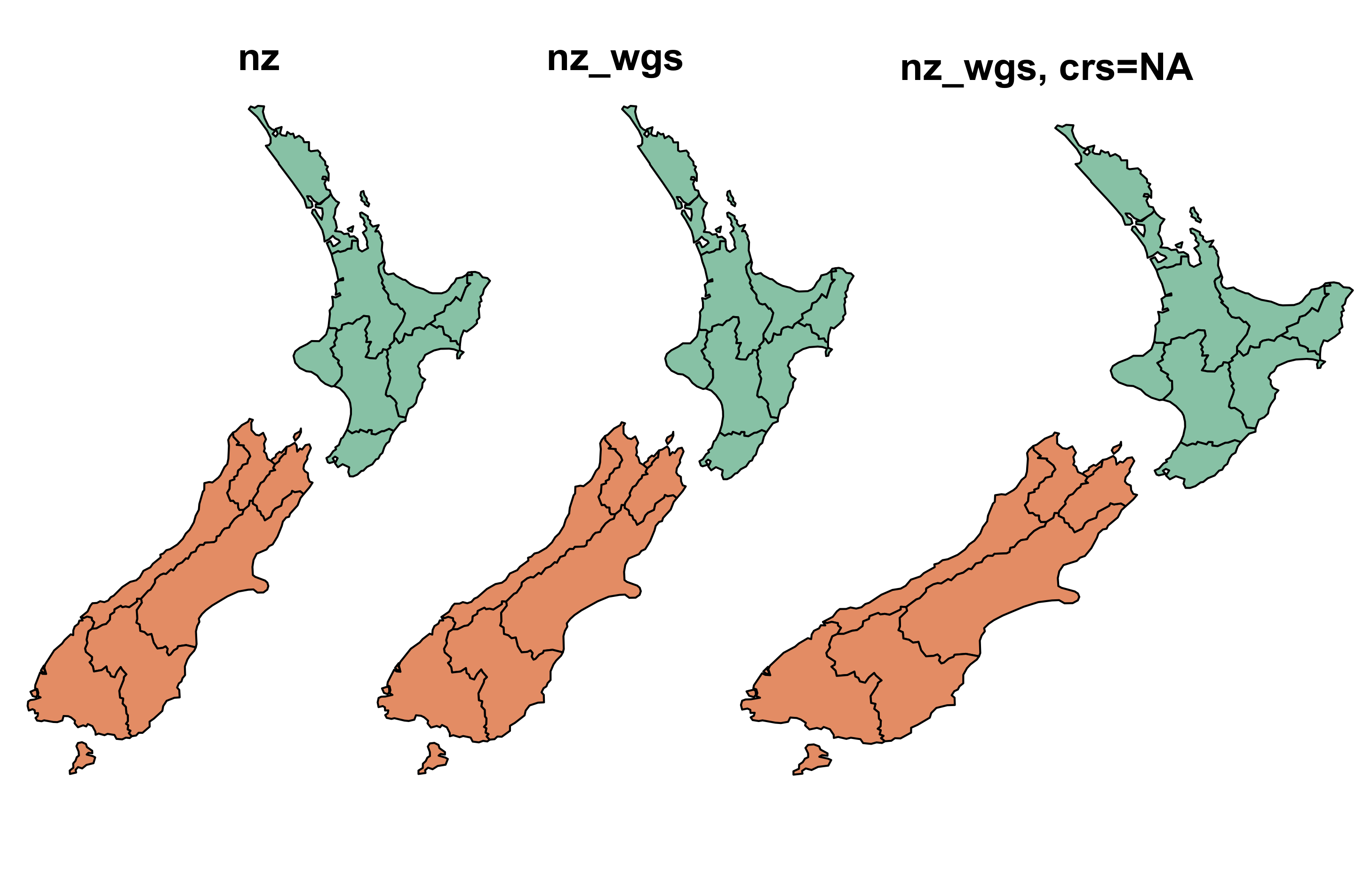
Create a new object called nz_wgs by transforming nz object into the WGS84 CRS.

Create an object of class crs for both and use this to query their CRSs.
With reference to the bounding box of each object, what units does each CRS use?
Remove the CRS from nz_wgs and plot the result: what is wrong with this map of New Zealand and why?

st_crs(nz)
# Coordinate Reference System:
#   EPSG: 2193 
#   proj4string: "+proj=tmerc +lat_0=0 +lon_0=173 +k=0.9996 +x_0=1600000 +y_0=10000000 +ellps=GRS80 +towgs84=0,0,0,0,0,0,0 +units=m +no_defs"
st_bbox(nz)
#    xmin    ymin    xmax    ymax 
# 1090144 4748537 2089533 6191874 
# 从 nz 的坐标参考的投影（proj4string）以及边界（st_bbox()）得知，其单位是 m ，即距离纬度为0°、经度为173°处的距离。

# WGS84坐标参考系的代码就是4326
nz_wgs <- st_transform(nz, crs=4326)
st_crs(nz_wgs)
# Coordinate Reference System:
#   EPSG: 4326 
#   proj4string: "+proj=longlat +datum=WGS84 +no_defs"
st_bbox(nz_wgs)
#      xmin      ymin      xmax      ymax 
# 166.42630 -47.28285 178.55037 -34.41452 
# 从 nz_wsg 的坐标参考的投影（proj4string）以及边界（st_bbox()）得知，其单位是 ° ，即经纬度，实际就是普遍用于地图的投影WGS84。

# 用 st_set_crs() 去掉 nz_wgs 的坐标参考系
nz_wgs_na <- st_set_crs(nz_wgs, NA)
# 注意函数 st_transform() 与 st_set_crs() 的区别
plot(nz["Island"], main = "nz")
plot(nz_wgs["Island"], main = "nz_wgs")
plot(nz_wgs_na["Island"], main = "nz_wgs, crs=NA")

Q2

Transform the world dataset to the transverse Mercator projection ("+proj=tmerc") and plot the result. What has changed and why? Try to transform it back into WGS 84 and plot the new object. Why does the new object differ from the original one?

world
# Simple feature collection with 177 features and 10 fields
# geometry type:  MULTIPOLYGON
# dimension:      XY
# bbox:           xmin: -180 ymin: -90 xmax: 180 ymax: 83.64513
# epsg (SRID):    4326
# proj4string:    +proj=longlat +datum=WGS84 +no_defs
# ...

world2 <- st_transform(world, crs = "+proj=tmerc")
world2
# Simple feature collection with 177 features and 10 fields (with 26 geometries empty)
# geometry type:  MULTIPOLYGON
# dimension:      XY
# bbox:           xmin: -15874400 ymin: -8733146 xmax: 14286950 ymax: 10884460
# epsg (SRID):    NA
# proj4string:    +proj=tmerc +lat_0=0 +lon_0=0 +k=1 +x_0=0 +y_0=0 +ellps=WGS84 +units=m +no_defs
# ...
plot(world2)
# 无法输出图像

world3 <- st_transform(world2, crs = 4326)
world3
# Simple feature collection with 177 features and 10 fields (with 26 geometries empty)
# geometry type:  MULTIPOLYGON
# dimension:      XY
# bbox:           xmin: -179.1856 ymin: -11087.25 xmax: 179.745 ymax: 1.345748e+14
# epsg (SRID):    4326
# proj4string:    +proj=longlat +datum=WGS84 +no_defs
# ...
# 这样转换坐标参考系之后再一次转换回去，有可能更改其值范围

Q3

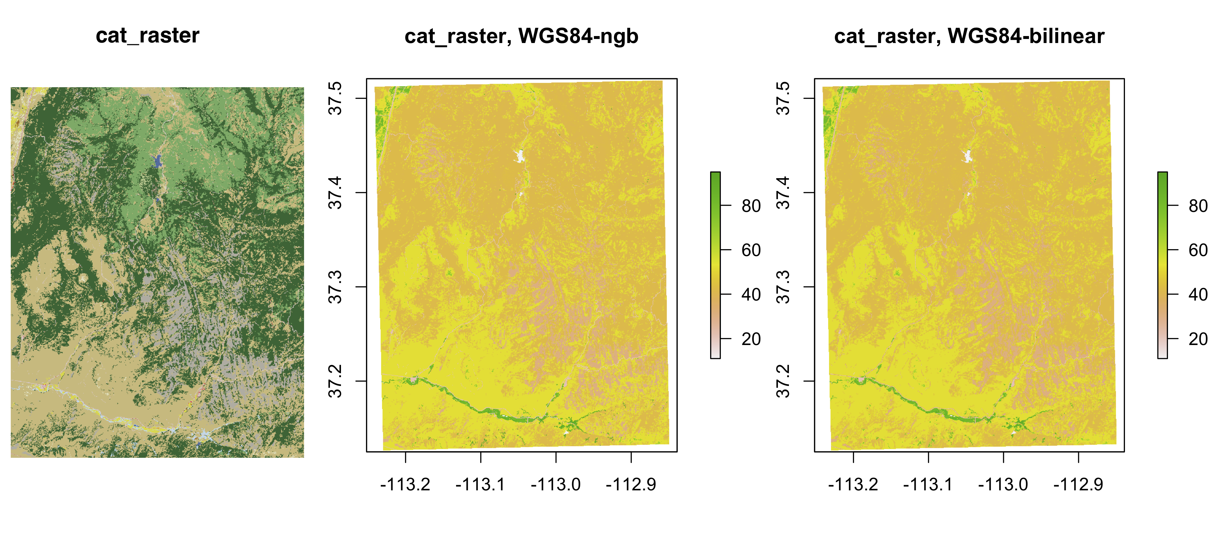
Transform the continuous raster (cat_raster) into WGS 84 using the nearest neighbor interpolation method. What has changed? How does it influence the results?

cat_raster = raster(system.file("raster/nlcd2011.tif", package = "spDataLarge"))
cat_raster
# class      : RasterLayer 
# dimensions : 1359, 1073, 1458207  (nrow, ncol, ncell)
# resolution : 31.5303, 31.52466  (x, y)
# extent     : 301903.3, 335735.4, 4111244, 4154086  (xmin, xmax, ymin, ymax)
# crs        : +proj=utm +zone=12 +ellps=GRS80 +towgs84=0,0,0,0,0,0,0 +units=m +no_defs 
# source     : /Library/Frameworks/R.framework/Versions/3.5/Resources/library/spDataLarge/raster/nlcd2011.tif 
# names      : nlcd2011 
# values     : 11, 95  (min, max)
cat_raster_ngb1 <- projectRaster(cat_raster, crs="+proj=longlat +datum=WGS84 +no_defs", method="ngb")
cat_raster_ngb1
# class      : RasterLayer 
# dimensions : 1394, 1111, 1548734  (nrow, ncol, ncell)
# resolution : 0.000356, 0.000284  (x, y)
# extent     : -113.2432, -112.8477, 37.12494, 37.52083  (xmin, xmax, ymin, ymax)
# crs        : +proj=longlat +datum=WGS84 +no_defs +ellps=WGS84 +towgs84=0,0,0 
# source     : memory
# names      : nlcd2011 
# values     : 11, 95  (min, max)
# 改变投影后，维度、分辨率（及其单位）、范围（及其单位）、投影等都发生了改变
plot(cat_raster, main = "cat_raster")
plot(cat_raster_ngb1, main = "cat_raster, WGS84")

Q4

Transform the categorical raster (cat_raster) into WGS 84 using the bilinear interpolation method. What has changed? How does it influence the results?

cat_raster_bilinear <- projectRaster(cat_raster, crs="+proj=longlat +datum=WGS84 +no_defs", method="bilinear")
cat_raster_bilinear
# class      : RasterLayer 
# dimensions : 1394, 1111, 1548734  (nrow, ncol, ncell)
# resolution : 0.000356, 0.000284  (x, y)
# extent     : -113.2432, -112.8477, 37.12494, 37.52083  (xmin, xmax, ymin, ymax)
# crs        : +proj=longlat +datum=WGS84 +no_defs +ellps=WGS84 +towgs84=0,0,0 
# source     : memory
# names      : nlcd2011 
# values     : 5.751417, 95  (min, max)
# 这是栅格值也发生了变化
plot(cat_raster_bilinear, main = "cat_raster, WGS84-bilinear")

Q5

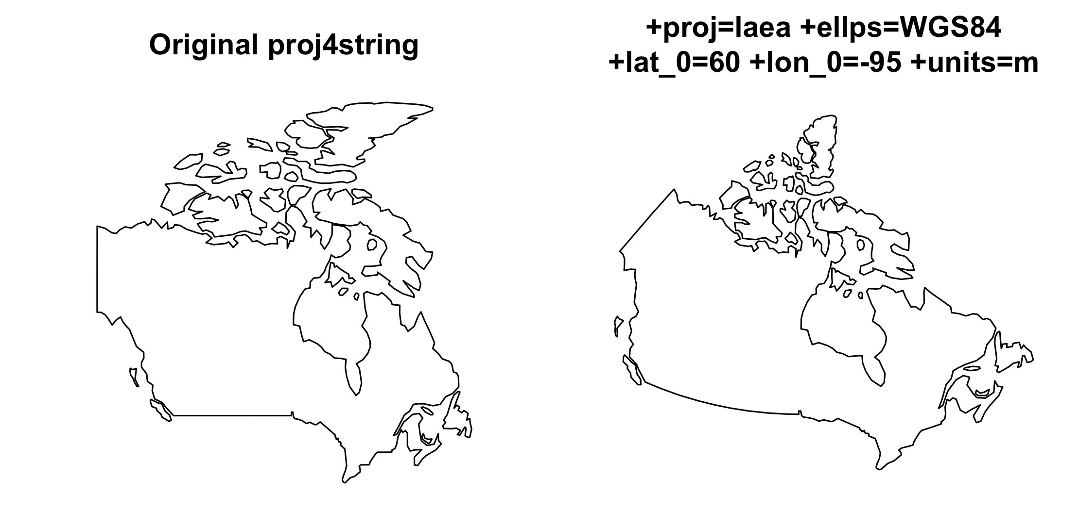
Create your own proj4string. It should have the Lambert Azimuthal Equal Area ( laea ) projection, the WGS84 ellipsoid, the longitude of projection center of 95 degrees west, the latitude of projection center of 60 degrees north, and its units should be in meters. Next, subset Canada from the world object and transform it into the new projection. Plot and compare a map before and after the transformation.

proj_new <- "+proj=laea +ellps=WGS84 +lat_0=60 +lon_0=-95 +units=m"
# 注意设置新投影时文本的格式
canada <- world %>% filter(name_long=="Canada")
canada_new <- st_transform(canada, crs=proj_new)
par(mfrow=c(1,2))
plot(st_geometry(canada), main="Original proj4string")
plot(st_geometry(canada_new), main="+proj=laea +ellps=WGS84 \n+lat_0=60 +lon_0=-95 +units=m")

原书习题答案详见Chapter 6: Reprojecting geographic data