The Geographic data I/O is mainly about reading (inputing) and writing (outputing) geographic data. They are important steps for geocomputation. This chapter introducted a lot of methods to access the online source of geographic data.
The exercise solutions could be accessed at Chapter 7: Geographic data I/O. Here I give the solutions with Chinese explainations.
解决问题
-
理解矢量、栅格数据的类型及文件格式(Q1)。
-
理解如何线上开源地图数据库中获取想要的空间地图数据
-
读入矢量文件(Q2)。
-
读入栅格文件(Q3)。
-
使用特定 R 程辑包下载或输入数据,并能输出数据(Q4&Q5)。
-
保存数据结果(Q4, Q5, Q6)
-
初步尝试网页交互地图数据显示(Q7)。
所需R包
library(sf)
library(raster)
library(dplyr)
library(spData)
Q1
List and describe three types of vector, raster, and geodatabase formats.
关于矢量、栅格的类型以及数据文件格式,可详细参考 Table 7.2
Q2
Name at least two differences between read_sf() and the more well-known function st_read().
?read_sf
?st_read
函数 read_sf() 的默认设置是 quiet=TRUE, stringsAsFactors = FALSE, as_tibble = TRUE ,而 st_read() 函数的默认设置是不一样的。 read_sf() 不输出数据源的信息,输出 sf-tibble 而不是 sf-data.frame 。详细参见两函数的各自帮助页面。
Q3
Read the cycle_hire_xy.csv file from the spData package as a spatial object (Hint: it is located in the misc\ folder). What is a geometry type of the loaded object?
cycle_hire <- system.file("misc/cycle_hire_xy.csv", package="spData")
cycle_hire_xy = st_read(cycle_hire, options = c("X_POSSIBLE_NAMES=X", "Y_POSSIBLE_NAMES=Y"))
cycle_hire_xy
# Simple feature collection with 742 features and 7 fields
# geometry type:  POINT
# dimension:      XY
# bbox:           xmin: -0.2367699 ymin: 51.45475 xmax: -0.002275 ymax: 51.54214
# epsg (SRID):    NA
# proj4string:    NA
# First 10 features:
#              X        Y id               name             area nbikes nempty
# 1  -0.10997053 51.52916  1       River Street      Clerkenwell      4     14
# 2  -0.19757425 51.49961  2 Phillimore Gardens       Kensington      2     34
# 3  -0.08460569 51.52128  3 Christopher Street Liverpool Street      0     32
# 4  -0.12097369 51.53006  4  St. Chad's Street     King's Cross      4     19
# 5  -0.15687600 51.49313  5     Sedding Street    Sloane Square     15     12
# 6  -0.14422888 51.51812  6 Broadcasting House       Marylebone      0     18
# 7  -0.16807430 51.53430  7   Charlbert Street  St. John's Wood     15      0
# 8  -0.17013448 51.52834  8         Lodge Road  St. John's Wood      5     13
# 9  -0.09644075 51.50739  9     New Globe Walk         Bankside      3     16
# 10 -0.09275416 51.50597 10        Park Street         Bankside      1     17
#                        geometry
# 1   POINT (-0.1099705 51.52916)
# 2   POINT (-0.1975742 51.49961)
# 3  POINT (-0.08460569 51.52128)
# 4   POINT (-0.1209737 51.53006)
# 5    POINT (-0.156876 51.49313)
# 6   POINT (-0.1442289 51.51812)
# 7    POINT (-0.1680743 51.5343)
# 8   POINT (-0.1701345 51.52834)
# 9  POINT (-0.09644075 51.50739)
# 10 POINT (-0.09275416 51.50597)
Q4
Download the borders of Germany using rnaturalearth, and create a new object called germany_borders. Write this new object to a file of the GeoPackage format.
library(rnaturalearth)
germany_border0 <- ne_countries(scale=10, country = "Germany")
germany_border <- st_as_sf(germany_border0)
plot(germany_border0, main="Germany Border")
# 或者
plot(st_geometry(germany_border), main="Germany Border")
# 写出生成的文件至工作文件夹
st_write(obj=germany_border, dsn="GermanyBorder.gpkg")

Q5
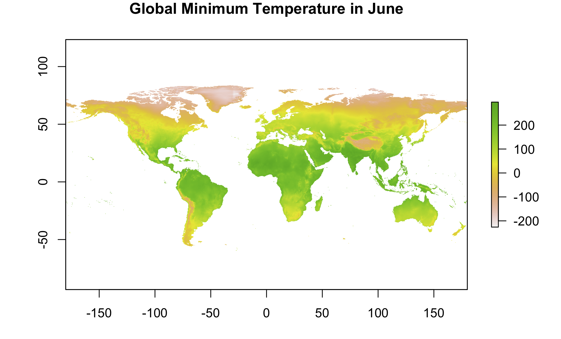
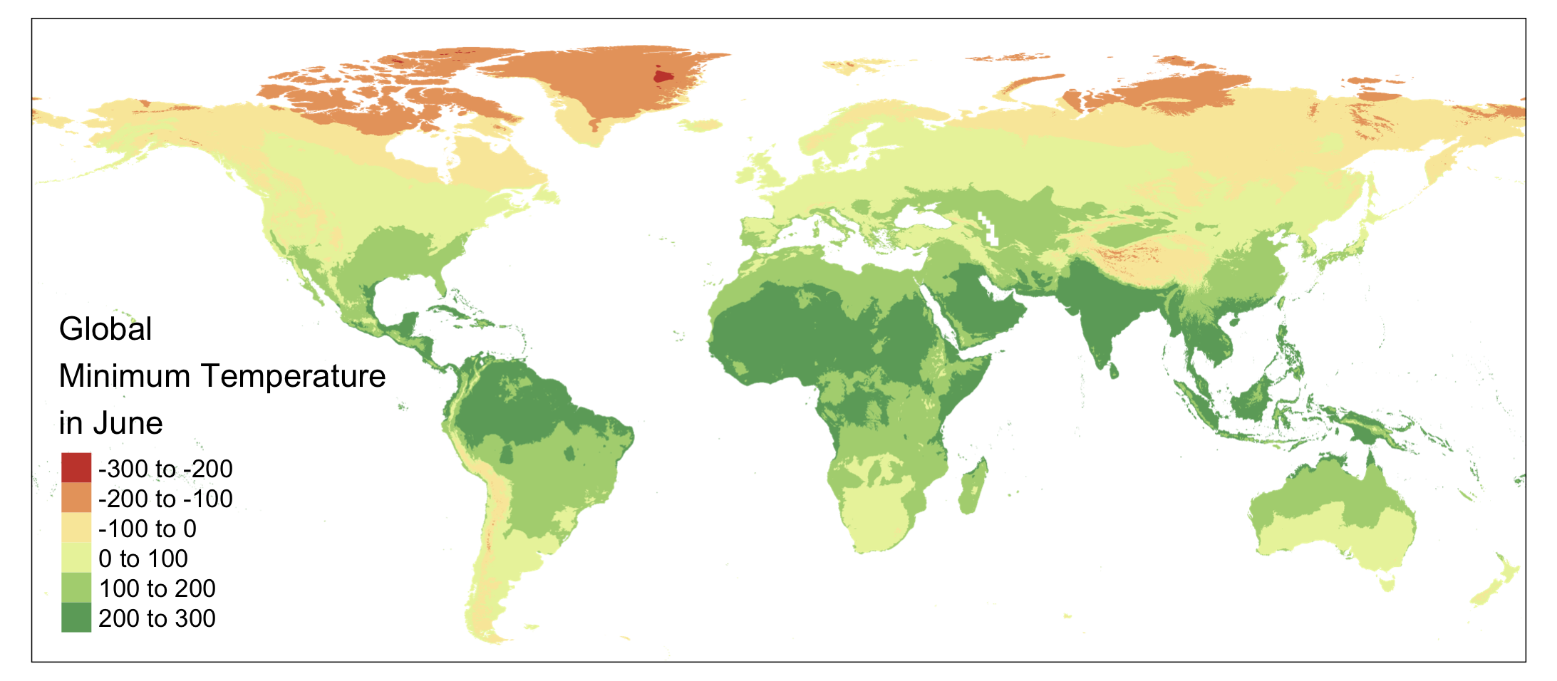
Download the global monthly minimum temperature with a spatial resolution of five minutes using the raster package. Extract the June values, and save them to a file named tmin_june.tif file (hint: use raster::subset() ).
tmin5 <- getData("worldclim", var = "tmin", res = 5)
# 将worldclim栅格数据下载到工作路径,设置 res = 5 即为空间分辨率为5分钟
# 从下载的文件包中得知,共有12个月的气温数据
tmin5_june <- raster::subset(tmin5, subset="tmin5", filename="tmin5_june.tif")
# 抽取其中的6月份的数据
plot(tmin5_june, legend=FALSE, main="Global Minimum Temperature in June")
# 用 tmap 程辑包可获得更美观的地图,详见第8章
library(tmap)
tmin5_june_map <- tm_shape(tmin5_june) + tm_raster(title = "Global\nMinimum Temperature\nin June") + tm_layout(legend.position = c("left", "bottom"))
tmin5_june_map
# 还可将 tmin5_june_map 保存到工作路径
tmap_save(tm = tmin5_june_plot, filename = "tmin5_june_map.png", dpi=300)
Q6
Create a static map of Germany’s borders, and save it to a PNG file.
png(filename = "Germany_Border.png")
plot(st_geometry(germany_border), main="Germany Border")
dev.off()
Q7
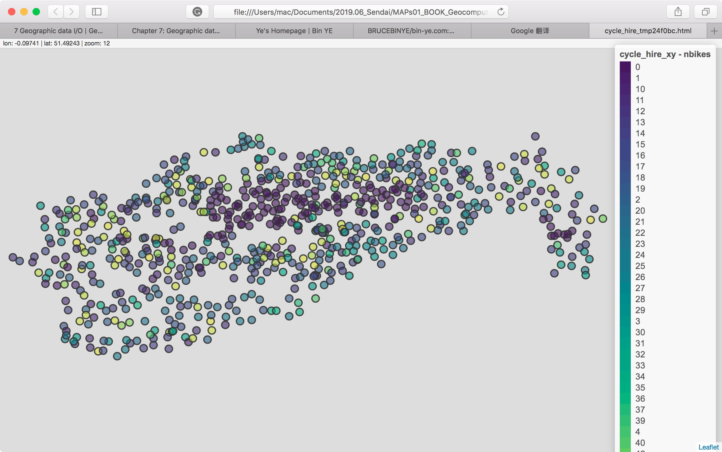
Create an interactive map using data from the cycle_hire_xy.csv file. Export this map to a file called cycle_hire.html.
cycle_hire <- system.file("misc/cycle_hire_xy.csv", package="spData")
cycle_hire_xy = st_read(cycle_hire, options = c("X_POSSIBLE_NAMES=X", "Y_POSSIBLE_NAMES=Y"))
# 初步创建交互网页地图
library(mapview)
# 输出数据为自行车数量 nbikes
cycle_hire_nbikes <- mapview(cycle_hire_xy, zcol="nbikes", legend=TRUE)
mapshot(cycle_hire_nbikes, file="cycle_hire.html")
原书习题答案请参见Chapter 7: Geographic data I/O。