Geocomputation with R - 05

The exercise solutions of Chapter 5 could be accessed at Chapter 5: Geometric operations. Here are solutions of mine explained in Chinese.

第五章继续讲述如何处理矢量对象（sf对象）和栅格对象的地理数据，以及矢量和栅格之间的交互、相互转换等。详细请阅读原文Geometry operations。习题参考答案如下。

解决问题

简化矢量数据，会根据实际需要，选取合适的简化方法（Q1）。
会使用 buffer 相关函数，计算与对象相关联的某一范围的信息（Q2）。
找出矢量对象（一般是多边形）的中心（Q3）。
对矢量对象（以及栅格对象）进行扩大、缩小、旋转、移动等处理（Q4）。
根据两个或多个对象的地理位置，取其交集、并集等（Q5）。
会对不同矢量对象进行转换（Q6）。
针对栅格对象，会使用相关的矢量对象，对其进行修剪和覆盖操作（Q7）。
针对栅格对象，会使用相关矢量对象，抽出与之相关的栅格值（Q8）。
会将矢量转换成栅格，会在转换过程中根据要求设置临时栅格，并会展示或抽取统计信息（Q9）。
减小或增大栅格对象的分辨率（Q10）。
会将栅格转换成矢量，并会展示或抽取其统计值（Q11）。

所需R包

library(sf)
library(raster)
library(dplyr)
library(spData)
library(spDataLarge)
library(rmapshaper)
library(RQGIS)

Q1

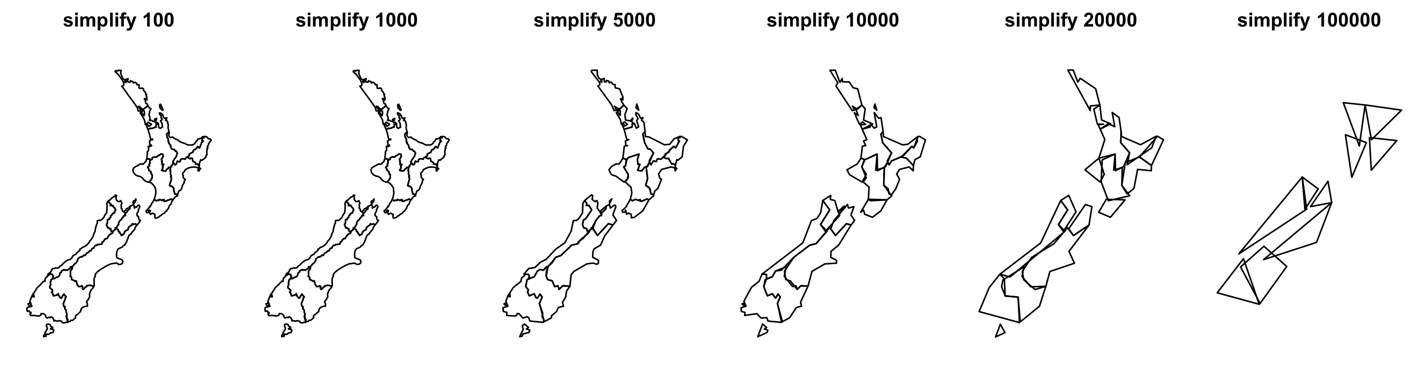
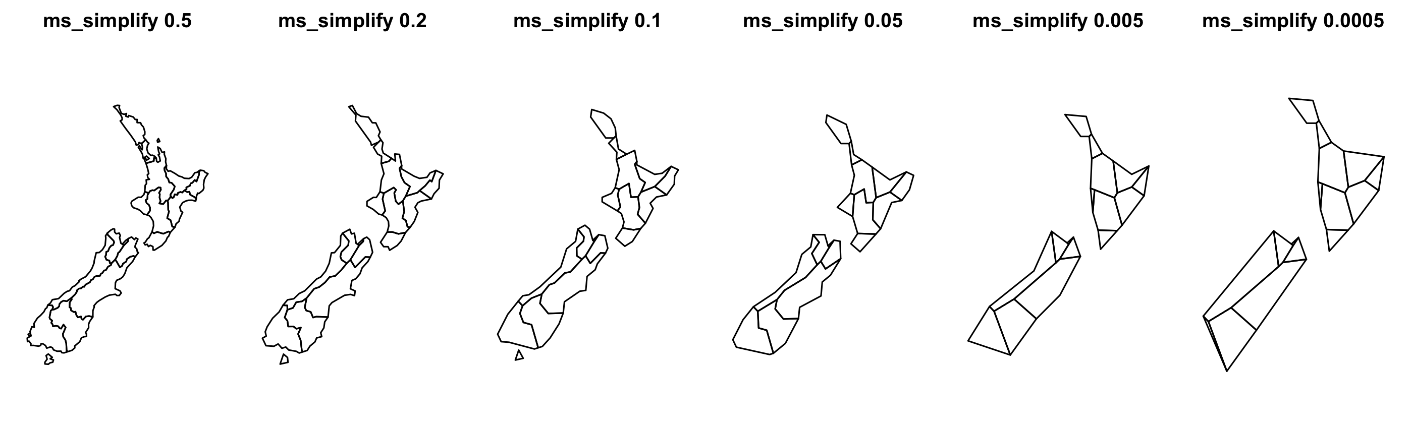
Generate and plot simplified versions of the nz dataset. Experiment with different values of keep (ranging from 0.5 to 0.00005) for ms_simplify() and dTolerance (from 100 to 100,000) st_simplify() .

At what value does the form of the result start to break down for each method, making New Zealand unrecognizable?
Advanced: What is different about the geometry type of the results from st_simplify() compared with the geometry type of ms_simplify() ? What problems does this create and how can this be resolved?

# 首先使用 st_simplify() 简化对象
nz.g <- st_geometry(nz)
nz_simple100 <- st_simplify(nz.g, dTolerance=100)
nz_simple1000 <- st_simplify(nz.g, dTolerance=1000)
nz_simple5000 <- st_simplify(nz.g, dTolerance=5000)
nz_simple10000 <- st_simplify(nz.g, dTolerance=10000)
nz_simple20000 <- st_simplify(nz.g, dTolerance=20000)
nz_simple100000 <- st_simplify(nz.g, dTolerance=100000)
par(mfrow = c(1,6), mar = c(0, 1, 2, 1))
plot(nz_simple100, main = "simplify 100")
plot(nz_simple1000, main = "simplify 1000")
plot(nz_simple5000, main = "simplify 5000")
plot(nz_simple10000, main = "simplify 10000")
plot(nz_simple20000, main = "simplify 20000")
plot(nz_simple100000, main = "simplify 100000")
# 以 nz_simple100 为例
nz_simple100
# geometry type:  GEOMETRY 
# 其几何类型是GEOMETRY

# 使用 rmapshaper::ms_simplify() 函数简化
library(rmapshaper)
nz_simple0.5 <- ms_simplify(nz.g, keep=0.5, keep_shapes=TRUE)
nz_simple0.2 <- ms_simplify(nz.g, keep=0.2, keep_shapes=TRUE)
nz_simple0.1 <- ms_simplify(nz.g, keep=0.1, keep_shapes=TRUE)
nz_simple0.05 <- ms_simplify(nz.g, keep=0.05, keep_shapes=TRUE)
nz_simple0.005 <- ms_simplify(nz.g, keep=0.005, keep_shapes=TRUE)
nz_simple0.0005 <- ms_simplify(nz.g, keep=0.0005, keep_shapes=TRUE)
par(mfrow = c(1,6), mar = c(0, 1, 2, 1))
plot(nz_simple0.5, main = "ms_simplify 0.5")
plot(nz_simple0.2, main = "ms_simplify 0.2")
plot(nz_simple0.1, main = "ms_simplify 0.1")
plot(nz_simple0.05, main = "ms_simplify 0.05")
plot(nz_simple0.005, main = "ms_simplify 0.005")
plot(nz_simple0.0005, main = "ms_simplify 0.0005")

# 以 nz_simple0.5 为例
nz_simple0.5
# geometry type:  MULTIPOLYGON
# 其几何类型为 MULTIPOLYGON 复合多边形

也就是说，使用 sf::st_simplify() 和 rmapshaper::ms_simplify() 得到的简化结果的几何类型是不同的。使用函数 st_cast() 将 GEOMETRY 类型转化为 MULTIPOLYGON 类型即可。

st_cast(nz_simple100, "MULTIPOLYGON")
# geometry type:  MULTIPOLYGON

Q2

In the first exercise in Chapter 4 it was established that Canterbury region had 70 of the 101 highest points in New Zealand. Using st_buffer() , how many points in nz_height are within 100 km of Canterbury?

canterbury <- nz %>% filter(Name == "Canterbury")
canterbury.buffer <- st_buffer(canterbury, dist = 100000)
canterbury.buffer.height <- nz_height[canterbury.buffer, ]
summarize(canterbury.buffer.height, n = n())
# Simple feature collection with 1 feature and 1 field
# geometry type:  MULTIPOINT
# dimension:      XY
# bbox:           xmin: 1234725 ymin: 5048309 xmax: 1654899 ymax: 5351665
# epsg (SRID):    2193
# proj4string:    +proj=tmerc +lat_0=0 +lon_0=173 +k=0.9996 +x_0=1600000 +y_0=10000000 +ellps=GRS80 +towgs84=0,0,0,0,0,0,0 +units=m +no_defs
#    n                       geometry
# 1 95 MULTIPOINT (1234725 5048309...
# 因此，在 Canterbury 周边的 buffer 为10km 时，共有95个高点

Q3

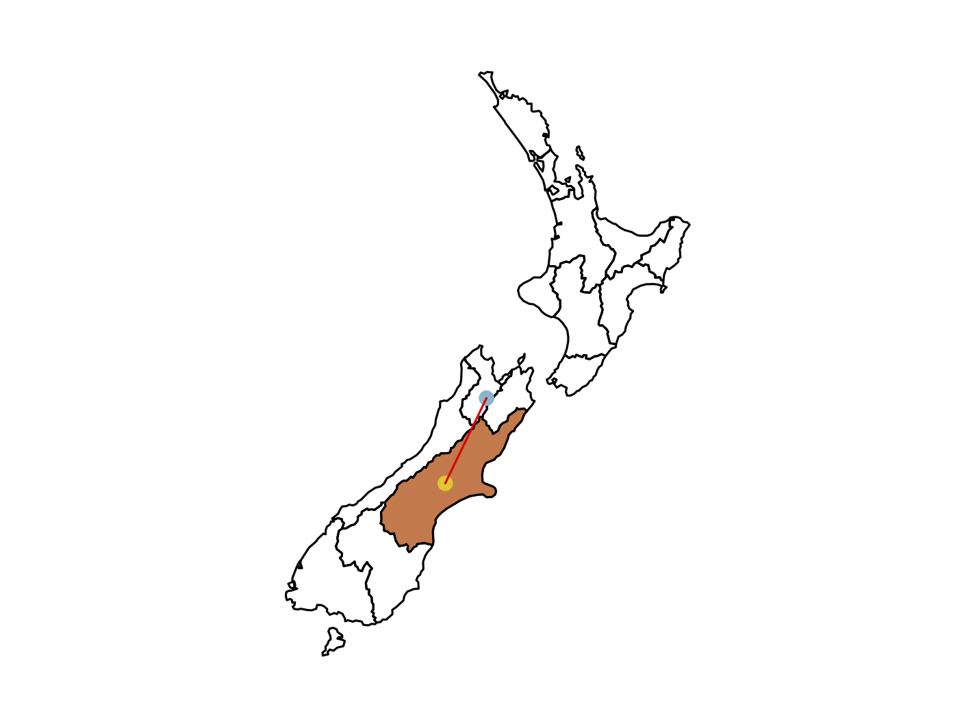
Find the geographic centroid of New Zealand. How far is it from the geographic centroid of Canterbury?

canterbury <- nz %>% filter(Name == "Canterbury")
nz.g <- st_geometry(nz)
# 将 nz 中各个地区统一成一个国家的边界，再找其中心
nz.union <- st_union(nz.g)
nz.cen <- st_centroid(nz.union)
# 找 canterbury 的中心
canterbury.cen <- st_centroid(canterbury)
st_distance(canterbury.cen, nz.cen)
# Units: [m]
#          [,1]
# [1,] 234192.6
# 两个中心之间的距离即为 234192.6 m
l <- st_linestring(rbind(c(1586811,5385284), c(1484732,5174509)))
par(mar = c(1,1,1,1))
plot(nz.g)
plot(st_geometry(canterbury), col = "#d87b48", add = TRUE)
plot(nz.cen, add = TRUE, col = "#78b4cc", pch=16)
plot(st_geometry(canterbury.cen), add = TRUE, col = "#e9c800", pch = 16)
plot(l, add = TRUE, col = "red")

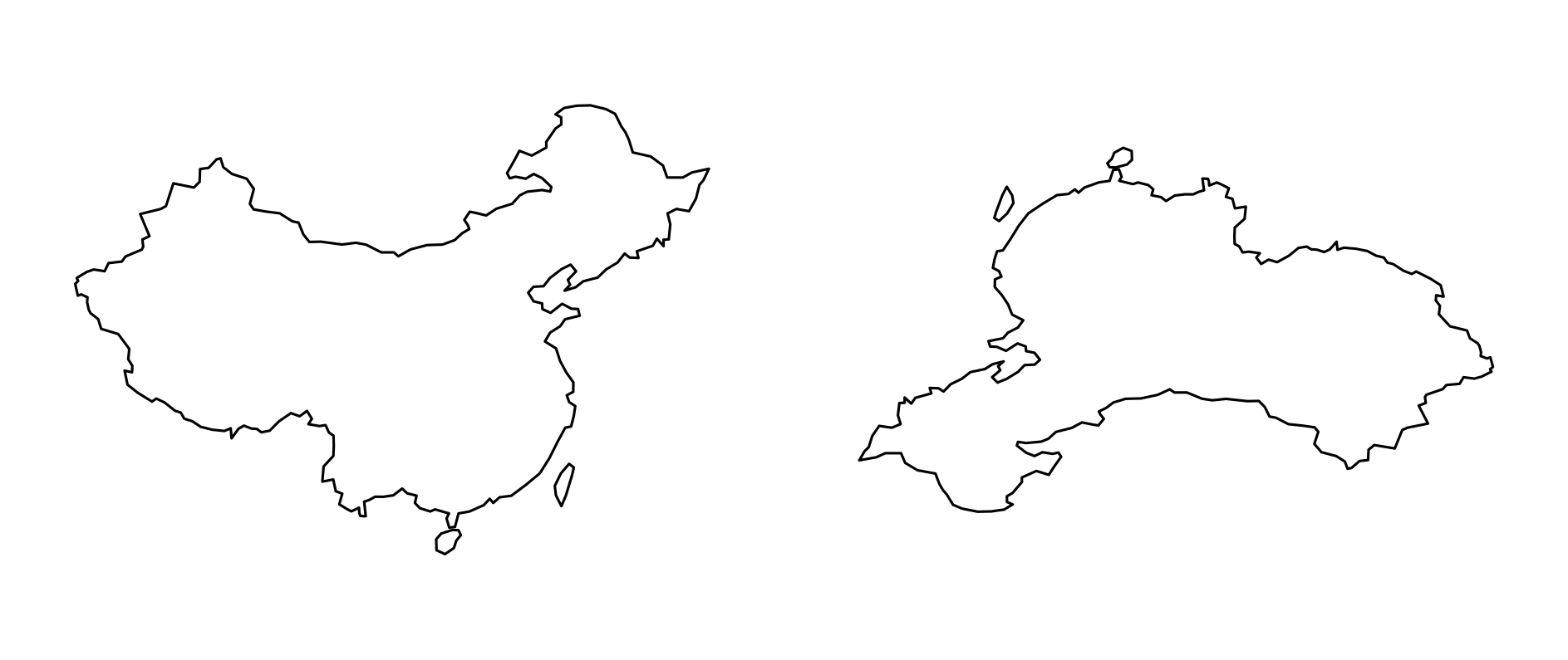
Q4

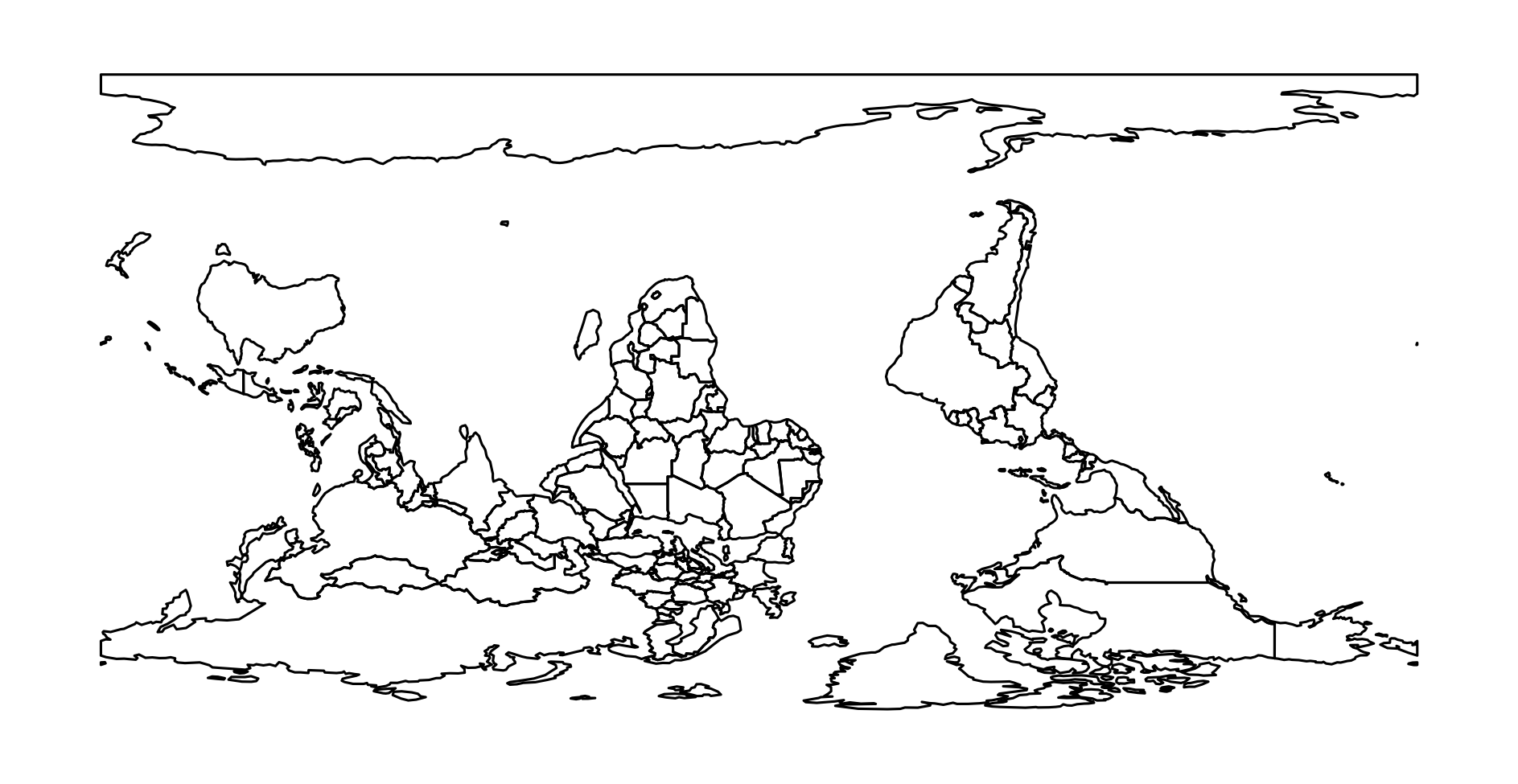
Most world maps have a north-up orientation. A world map with a south-up orientation could be created by a reflection (one of the affine transformations not mentioned in Section 5.2.4) of the world object’s geometry. Write code to do so. Hint: you need to use a two-element vector for this transformation.

Bonus: create an upside-down map of your country.

rotation = function(a){
  r = a * pi / 180 #degrees to radians
  matrix(c(cos(r), sin(r), -sin(r), cos(r)), nrow = 2, ncol = 2)
}
world.g <- st_geometry(world)
world.g.rotate <- world.g * rotation(180)
plot(world.g.rotate)

china <- world %>% filter(iso_a2 == "CN" | iso_a2 == "TW")
china.g <- st_geometry(china)
china.rotate <- china.g * rotation(180)
plot(china.g)
plot(china.rotate)

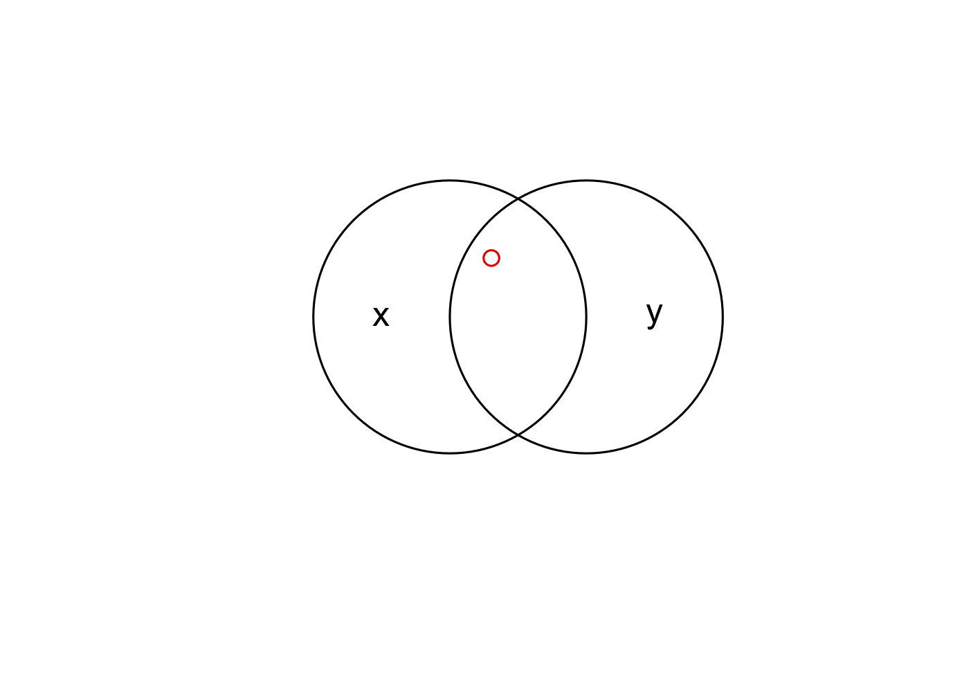
Q5

Subset the point in p that is contained within x and y (see Section 5.2.5 and Figure 5.8). Using base subsetting operators. Using an intermediary object created with st_intersection() .

b = st_sfc(st_point(c(0, 1)), st_point(c(1, 1))) # create 2 points
b = st_buffer(b, dist = 1) # convert points to circles
plot(b)
text(x = c(-0.5, 1.5), y = 1, labels = c("x", "y")) # add text
x = b[1]
y = b[2]
x_and_y = st_intersection(x, y)

bb = st_bbox(st_union(x, y))
box = st_as_sfc(bb)
set.seed(2017)
p = st_sample(x = box, size = 10)
sel_p_xy = st_intersects(p, x, sparse = FALSE)[, 1] & st_intersects(p, y, sparse = FALSE)[, 1]
p_xy1 = p[sel_p_xy]
plot(p_xy1, add = TRUE, col = "red")

Q6

Calculate the length of the boundary lines of US states in meters. Which state has the longest border and which has the shortest? Hint: The st_length function computes the length of a LINESTRING or MULTILINESTRING geometry.

data(us_states)
us <- st_union(us_states) %>% st_sf()
# 将所有州合并为一个国家
us.border <- st_cast(us, "MULTILINESTRING")
length(us.border)
# 24086689 [m]

# 计算每个州的边界长度，直接将其作为 us_states 的新一列数据
us_states$border.length <- st_length(us_states)
us_states
minborder <- us_states %>% filter(border.length == min(border.length))
maxborder <- us_states %>% filter(border.length == max(border.length))
minborder
# Simple feature collection with 1 feature and 7 fields
# geometry type:  MULTIPOLYGON
# dimension:      XY
# bbox:           xmin: -77.11976 ymin: 38.79165 xmax: -76.90939 ymax: 38.99555
# epsg (SRID):    4269
# proj4string:    +proj=longlat +datum=NAD83 +no_defs
#   GEOID                 NAME REGION          AREA total_pop_10 total_pop_15
# 1    11 District of Columbia  South 178.21 [km^2]       584400       647484
#   border.length                       geometry
# 1  60268.39 [m] MULTIPOLYGON (((-77.11976 3...
# 因此州边界最短的是 Columbia, 60268.39 m
maxborder
# Simple feature collection with 1 feature and 7 fields
# geometry type:  MULTIPOLYGON
# dimension:      XY
# bbox:           xmin: -106.6359 ymin: 25.84012 xmax: -93.51694 ymax: 36.50044
# epsg (SRID):    4269
# proj4string:    +proj=longlat +datum=NAD83 +no_defs
#   GEOID  NAME REGION            AREA total_pop_10 total_pop_15
# 1    48 Texas  South 687714.3 [km^2]     24311891     26538614
#   border.length                       geometry
# 1   4957325 [m] MULTIPOLYGON (((-103.0024 3...
# 因此州边界最长的是 Texas, 4957325 m

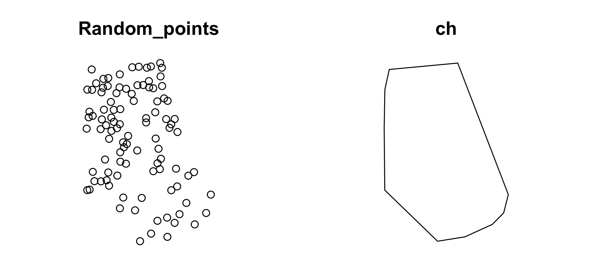
Q7

Crop the ndvi raster using (1) the random_points dataset and (2) the ch dataset. Are there any differences in the output maps? Next, mask ndvi using these two datasets. Can you see any difference now? How can you explain that?

# ch 对象
multi_random_points <- st_combine(random_points) # MULTIPOINTS
convexhull <- st_convex_hull(multi_random_points) # Convex Hull of multipoints
ch <- convexhull
data(random_points)
par(mfrow = c(1,2))
plot(st_geometry(random_points), main = "Random_points")
plot(ch, main = "ch")

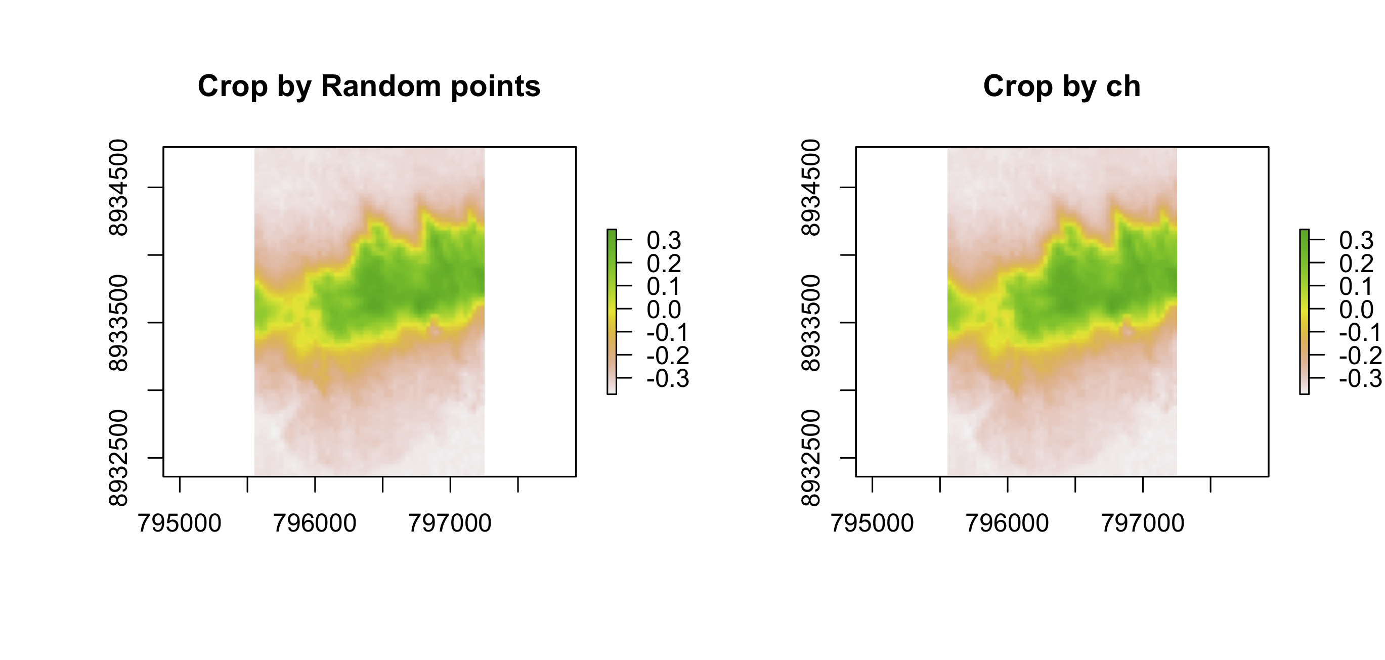
Crop （修剪）栅格 ndvi:

data(ndvi)
random_points <- st_transform(random_points, crs=projection(ndvi))
rp_ndvi_crop <- crop(ndvi, random_points)
ch <- st_transform(ch, crs=projection(ndvi)) %>% st_sf()
ch_ndvi_crop <- crop(ndvi, ch)

par(mfrow = c(1,2))
plot(rp_ndvi_crop, main = "Crop by Random points")
plot(ch_ndvi_crop, main = "Crop by ch")
all.equal(ch_ndvi_crop, rp_ndvi_crop)
# [1] TRUE
# 结果说明两者的 crop 栅格是相同的

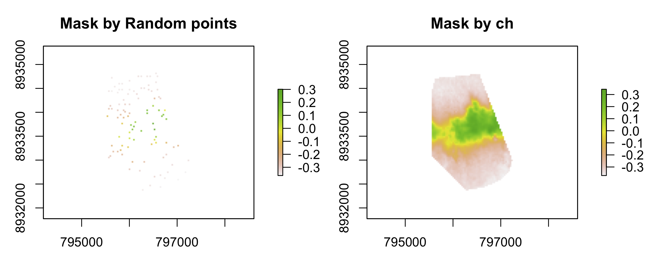
Mask （覆盖）栅格 ndvi:

rp_ndvi_mask <- mask(ndvi, random_points)
ch_ndvi_mask <- mask(ndvi, ch)
all.equal(ch_ndvi_mask, rp_ndvi_mask)
# [1] FALSE
# Warning message:
# In compareRaster(target, current, ..., values = values, stopiffalse = stopiffalse,  :
#   not all objects have the same values
# 因此可以发现，覆盖 Mask 与修剪 Crop 的结果是完全不同的。
par(mfrow = c(1,2))
plot(rp_ndvi_mask, main = "Mask by Random points")
plot(ch_ndvi_mask, main = "Mask by ch")

Q8

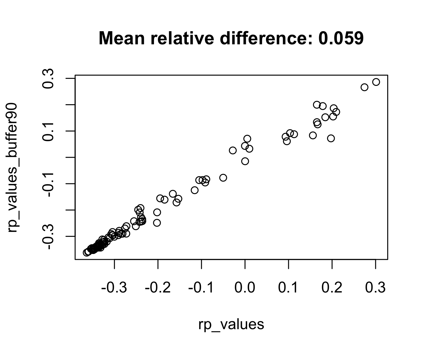
Firstly, extract values from ndvi at the points represented in random_points. Next, extract average values of ndvi using a 90 buffer around each point from random_points and compare these two sets of values. When would extracting values by buffers be more suitable than by points alone?

rp_values <- extract(ndvi, random_points)
rp_values_buffer90 <- extract(ndvi, random_points, buffer = 90, fun = mean)
all.equal(rp_values_buffer90, rp_values)
# [1] "Mean relative difference: 0.05919423"
# 将由两种方法抽出的值画出相关关系
plot(rp_values, rp_values_buffer90, main = "Mean relative difference: 0.059")

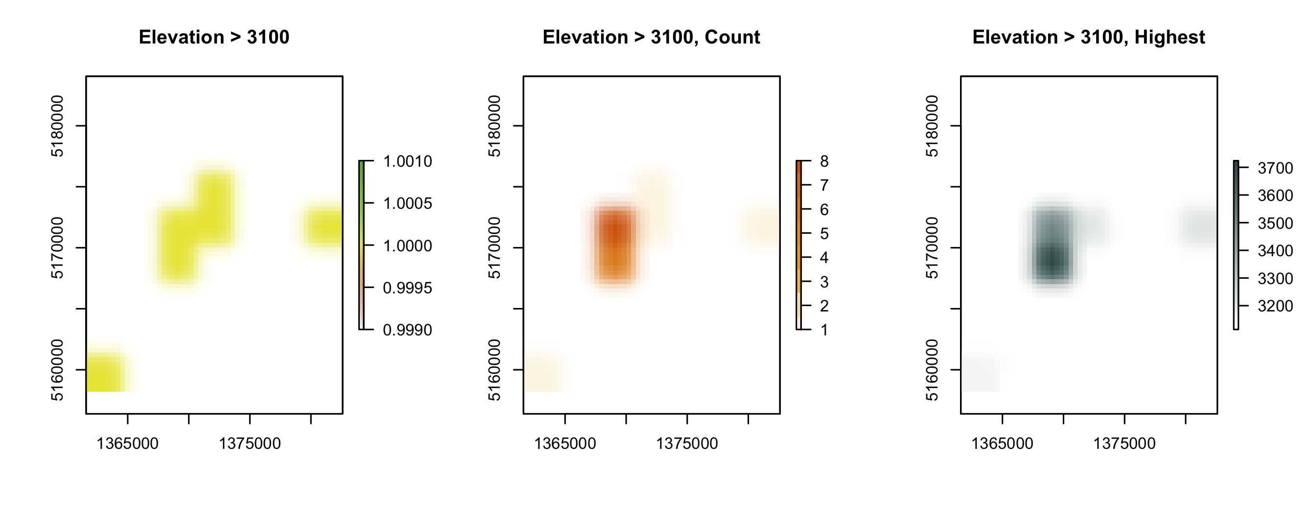
Q9

Subset points higher than 3100 meters in New Zealand (the nz_height object) and create a template raster with a resolution of 3 km. Using these objects:

Count numbers of the highest points in each grid cell.
Find the maximum elevation in each grid cell.

data(nz_height)
# 提出海拔高于3100 m 的值及其点
nz_height_h3100 <- nz_height %>% filter(elevation >= 3100)
nz_height_h3100
# Simple feature collection with 19 features and 2 fields
# geometry type:  POINT
# dimension:      XY
# bbox:           xmin: 1361593 ymin: 5159139 xmax: 1383924 ymax: 5182220
# epsg (SRID):    2193
# proj4string:    +proj=tmerc +lat_0=0 +lon_0=173 +k=0.9996 +x_0=1600000 +y_0=10000000 +ellps=GRS80 +towgs84=0,0,0,0,0,0,0 +units=m +no_defs
# First 10 features:
#    t50_fid elevation                geometry
# 1  2363993      3114 POINT (1372062 5173236)
# 2  2364015      3199 POINT (1382336 5173201)
# 3  2364239      3109 POINT (1383924 5182220)
# 4  2372186      3151 POINT (1361593 5159139)
# 5  2372234      3593 POINT (1369178 5167611)
# 6  2372235      3717 POINT (1369513 5168236)
# 7  2372236      3724 POINT (1369318 5169132)
# 8  2372237      3440 POINT (1369117 5169750)
# 9  2372252      3688 POINT (1369382 5168762)
# 10 2372292      3198 POINT (1368235 5169922)
# 将这些矢量点 point 转化为栅格，需要首先定义一个临时栅格
ras_tem <- raster(extent(nz_height_h3100), resolution=3000, crs= st_crs(nz_height_h3100$proj4string))
# 将这些矢量点 point 转化为栅格
nz_height_h3100_r1 <- rasterize(nz_height_h3100, ras_tem, field=1)
plot(nz_height_h3100_r1, main = "Elevation > 3100") # 左图

# 将转化的栅格中的值，定义成每个cell 包含的点（高于3100米）的数量
nz_height_h3100_r2 <- rasterize(nz_height_h3100, ras_tem, field=1, fun="count")
plot(nz_height_h3100_r2, main = "Elevation > 3100, Count", col=c("#fff3e0","#ffe0b2","#ffb740","#ff9800","#fb8c00","#f57c00","#ef6c00","#e65100")) 
# 中图

# 将转化的栅格中的值，定义成每个cell 中最高点的高度
nz_height_h3100_r3 <- rasterize(nz_height_h3100, ras_tem, field="elevation", fun="max")
plot(nz_height_h3100_r3, main = "Elevation > 3100, Highest", col = colorRampPalette(c("white", "#104641"))(256)) 
# 右图

Q10

Aggregate the raster counting high points in New Zealand (created in the previous exercise), reduce its geographic resolution by half (so cells are 6 by 6 km) and plot the result.

Resample the lower resolution raster back to a resolution of 3 km. How have the results changed?
Name two advantages and disadvantages of reducing raster resolution.

nz_height_h3100_r2
# class      : RasterLayer 
# dimensions : 8, 7, 56  (nrow, ncol, ncell)
# resolution : 3000, 3000  (x, y)  # 分辨率为3000 m，即3 km
# extent     : 1361593, 1382593, 5158220, 5182220  (xmin, xmax, ymin, ymax)
# crs        : NA 
# source     : memory
# names      : layer 
# values     : 1, 8  (min, max)
agg1 <- aggregate(nz_height_h3100_r2, fact=2, fun=mean)
agg1 # 使用 fact = 2 降低分辨率一半
# class      : RasterLayer 
# dimensions : 4, 4, 16  (nrow, ncol, ncell)
# resolution : 6000, 6000  (x, y)
# extent     : 1361593, 1385593, 5158220, 5182220  (xmin, xmax, ymin, ymax)
# crs        : NA 
# source     : memory
# names      : layer 
# values     : 1, 6  (min, max)
plot(agg1, main = "Half Resolution", col=c("#fff3e0","#ffe0b2","#ffb740","#ff9800","#fb8c00","#f57c00"))
# 左图

resample1 <- resample(agg1, nz_height_h3100_r2)
resample1
# class      : RasterLayer 
# dimensions : 8, 7, 56  (nrow, ncol, ncell)
# resolution : 3000, 3000  (x, y)
# extent     : 1361593, 1382593, 5158220, 5182220  (xmin, xmax, ymin, ymax)
# crs        : NA 
# source     : memory
# names      : layer 
# values     : -0.25, 6  (min, max)
plot(resample1, main = "Resample to Resolution")
# 右图

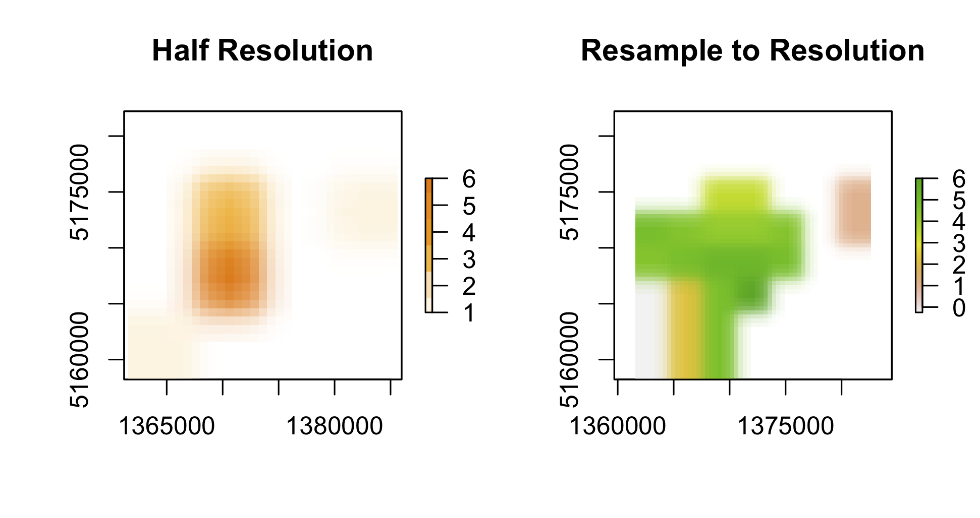
因此，对于某一栅格，降低分辨率后，优点是栅格文件会更小更便于快速计算，缺点是新的栅格值有所改变，并细节化程度降低。如果试图从降低分辨率之后的栅格再增加分辨率回到原来的分辨率，有可能产生跟原始分辨率的栅格完全不同的结果。

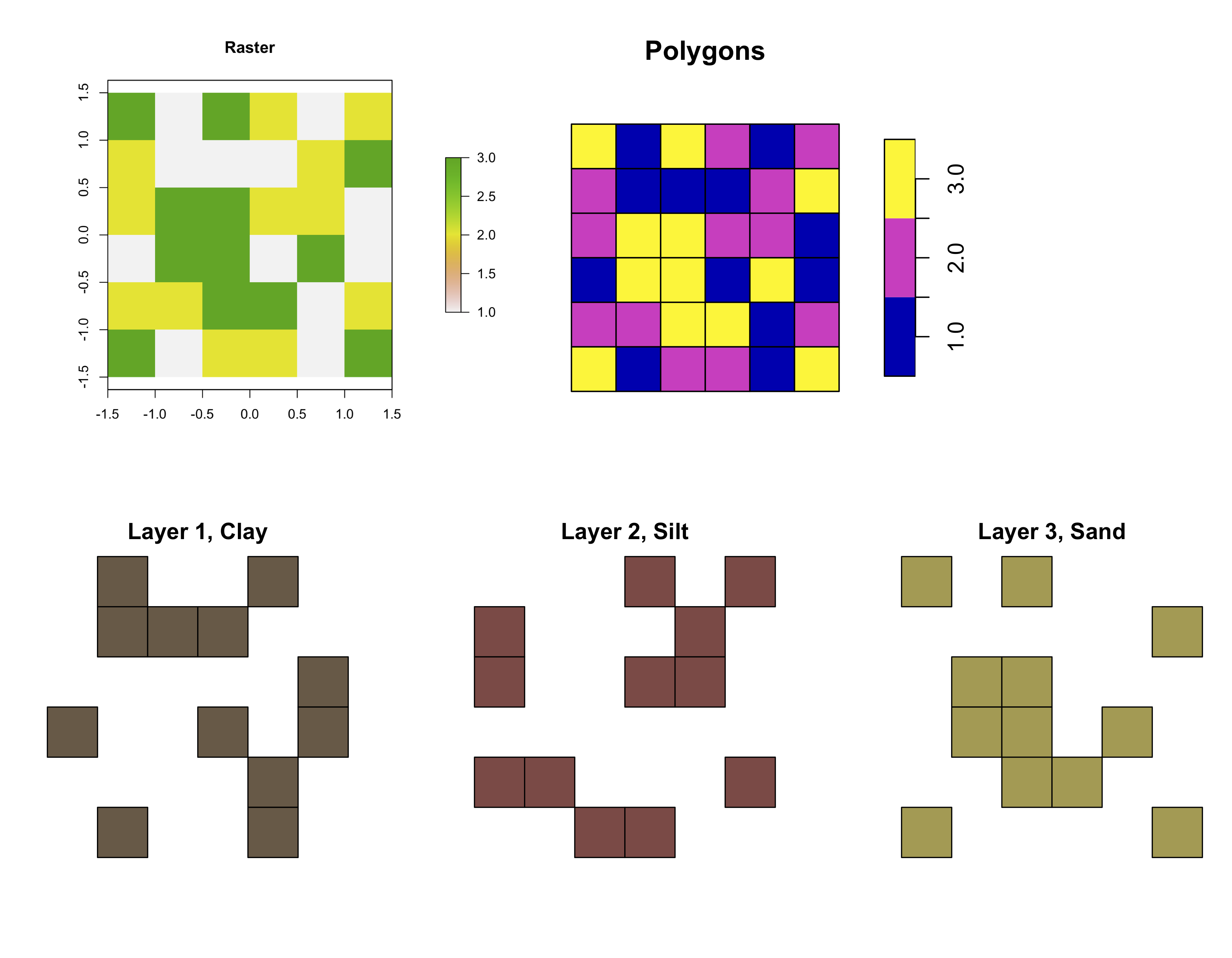
Q11

Polygonize the grain dataset and filter all squares representing clay.

Name two advantages and disadvantages of vector data over raster data.
At which points would it be useful to convert rasters to vectors in your work?

grain
# class      : RasterLayer 
# dimensions : 6, 6, 36  (nrow, ncol, ncell)
# resolution : 0.5, 0.5  (x, y)
# extent     : -1.5, 1.5, -1.5, 1.5  (xmin, xmax, ymin, ymax)
# crs        : +proj=longlat +datum=WGS84 +ellps=WGS84 +towgs84=0,0,0 
# source     : memory
# names      : layer 
# values     : 1, 3  (min, max)
# attributes :
#  ID VALUE
#   1  clay
#   2  silt
#   3  sand
# 将栅格转化为矢量
grain_polygon <- rasterToPolygons(grain) %>% st_as_sf()
#分别选取各个类别的值所代表的多边形
grain_polygon1 <- grain_polygon %>% filter(layer == 1)
grain_polygon2 <- grain_polygon %>% filter(layer == 2)
grain_polygon3 <- grain_polygon %>% filter(layer == 3)
plot(grain, main = "Raster")
plot(grain_polygon, main = "Polygons")
plot(grain_polygon1, main = "Layer 1, Clay", col = "#6c5844")
plot(grain_polygon2, main = "Layer 2, Silt", col = "#894944")
plot(grain_polygon3, main = "Layer 3, Sand", col = "#a89b4e")

原书习题参考答案详见Chapter 5: Geometric operations。