The exercise solutions of Chapter 4 could be accessed at Chapter 4: Spatial operations. Here are solutions of mine explained in Chinese.
第四章 Spatial data operations 讲述了地理计算中必不可少的内容,即空间数据操作,包括对矢量和栅格对象中的地理数据的不同处理方法。针对矢量数据(Vector)的空间操作包括:空间取亚集(Spatial subsetting)、几何形状之间的拓扑关系(Topological relations)、空间合并(Spatial joining)及非重叠合并(Ono-overlap joining)、空间数据集成统计(Spatial data aggregation)及空间距离关系(Distance relations),详见章节4.2。针对栅格数据(Raster)的空间操作包括:空间取亚集(Spatial subseting)、地图代数(Map algebra)、当地-焦点-区域-全局的空间操作(Local-Focal-Zonal-Global operations)、栅格地图代数操作与矢量操作的对应性(Map algebra counterparts in vector processing)、栅格合并(Merging rasters),详见章节4.3。
两种类型地理数据对象的空间处理具有相似性,也有各自的特点。在R中很容易区分,即一般用 sf 程辑包、其中以 st_ 开头的函数都是用于处理矢量数据对象的,而用于栅格数据对象的则一般是 raster 程辑包。
第四章习题原版答案请参见Chapter 4: Spatial operations,这里仅列出本人学完本章之后做出的习题答案,仅供对比参考。
解决问题
-
依据矢量对象地理数据的关联性,整合两个矢量数据或后续提取数据(Q1)。
-
依据矢量对象的地理数据,进行数据统计(Q2,Q3)。
-
对连续数据栅格对象,根据条件进行重分类(Q4)。
-
对栅格数据进行 local, focal, global 操作(Q5)。
-
根据栅格对象的值,进行地图代数计算(Q6)。
-
使用栅格覆盖(mask)、地图代数、数据统计整合起来,计算复杂问题,如计算陆地上的每一点距离海岸线的距离(Q7)。
所需R包
library(sf)
library(raster)
library(dplyr)
library(spData)
library(RQGIS)
library(spDataLarge)
library(maptools)
Q1
It was established in Section 4.2 that Canterbury was the region of New Zealand containing most of the 100 highest points in the country. How many of these high points does the Canterbury region contain?
data(nz)  # 新西兰地图
data(nz_height)  # 新西兰的高山
# 将 Canterbury 这一区域提出出来
can <- nz %>% filter(Name == "Canterbury")
# 将nz_height 中对应于 Canterbury 的地理数据抽出来
can_height <- nz_height[can, ]
nrow(can_height)
# [1] 70
Q2 & Q3
Which region has the second highest number of nz_height points in, and how many does it have?
Generalizing the question to all regions: how many of New Zealand’s 16 regions contain points which belong to the top 100 highest points in the country? Which regions?
Bonus: create a table listing these regions in order of the number of points and their name.
# 用 summarize() 函数中的 count=n() 统计落在同一地区内的点的个数
height <- st_join(nz, nz_height) %>%
  group_by(Name) %>%
  summarize(count=n())
# 按照个数多少排列
q3.count <- st_drop_geometry(height)
attach(q3.count)
q3.count.order <- q3.count[order(-count),]
q3.count.order
# # A tibble: 16 x 2
#    Name              count
#    <chr>             <int>
#  1 Canterbury           70
#  2 West Coast           22
#  3 Waikato               3
#  4 Manawatu-Wanganui     2
#  5 Otago                 2
#  6 Auckland              1
#  7 Bay of Plenty         1
#  8 Gisborne              1
#  9 Hawke's Bay           1
# 10 Marlborough           1
# 11 Nelson                1
# 12 Northland             1
# 13 Southland             1
# 14 Taranaki              1
# 15 Tasman                1
# 16 Wellington            1
# 因此,高山数量第二多的地区是 West Coast。每一个地区的高山数量也列出来了。
Q4
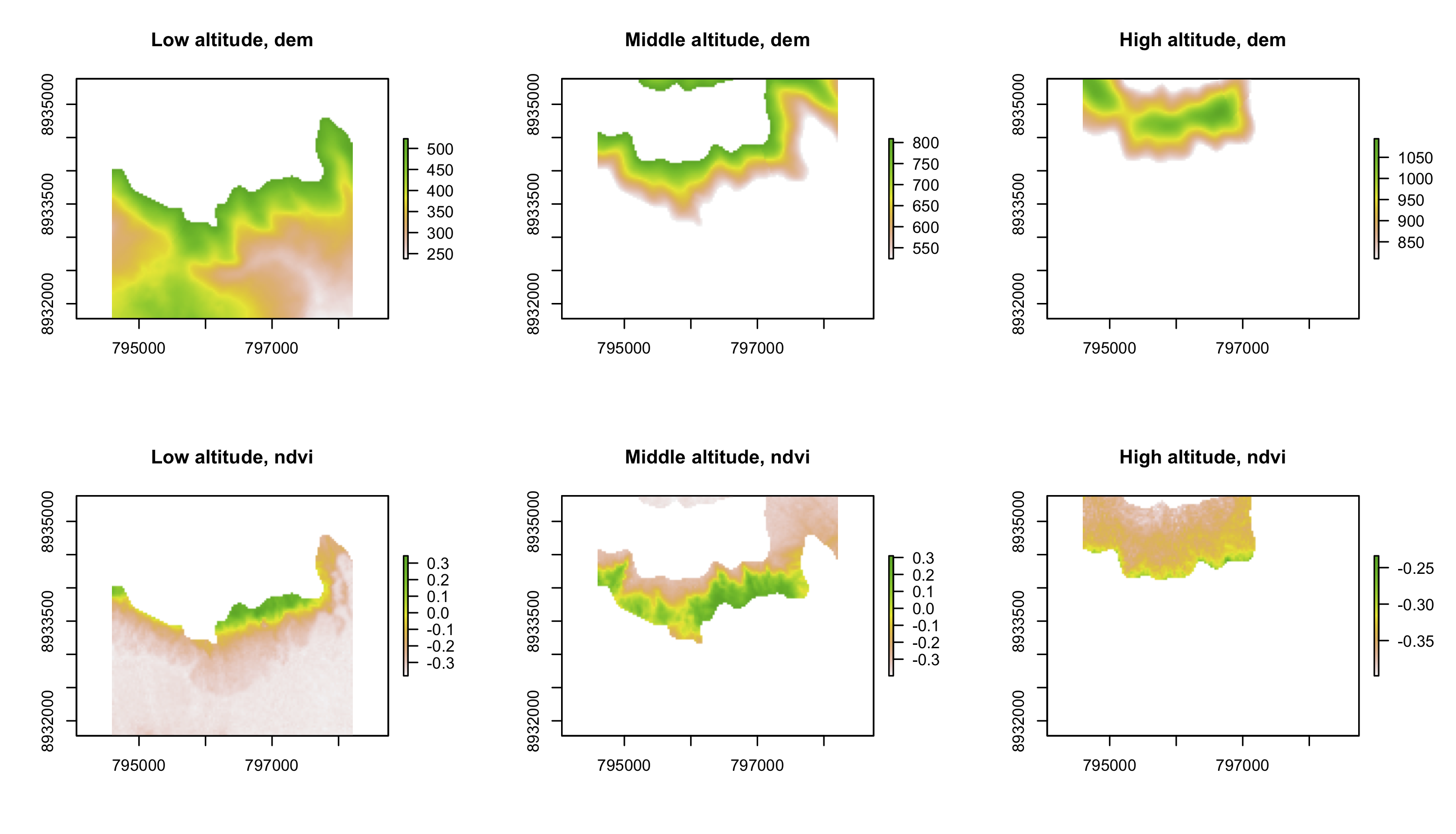
Use data(dem, package = "RQGIS"), and reclassify the elevation in three classes: low, medium and high. Secondly, attach the NDVI raster ( data(ndvi, package = "RQGIS") ) and compute the mean NDVI and the mean elevation for each altitudinal class.
data(dem, package = "RQGIS")
data(ndvi, package = "RQGIS")
dem
# class      : RasterLayer
# dimensions : 117, 117, 13689  (nrow, ncol, ncell)
# resolution : 30.85, 30.85  (x, y)
# extent     : 794599.1, 798208.6, 8931775, 8935384  (xmin, xmax, ymin, ymax)
# crs        : +proj=utm +zone=17 +south +ellps=WGS84 +towgs84=0,0,0,0,0,0,0 +units=m +no_defs
# source     : memory
# names      : dem
# values     : 238, 1094  (min, max)
# 可以看到 dem 栅格对象的值范围是238-1094,因此根据这一海拔高度值的范围,分为三类
m <- c(238,523,1, 523,809,2, 809,1094,3)
rcl <- matrix(m, ncol=3, byrow=TRUE)
dem_new <- reclassify(dem, rcl=rcl, include.lowest = TRUE)
# 如果这里定义include.lowest = FALSE,则需要将分类矩阵的最小起始值减1,即237~523
plot(dem_new, col=c("#e4beaa", "#b26a5e", "#910714"))

# 在新定义的栅格图层dem_new的区域内,计算 dem 和 ndvi 的相应值的统计平均
zonal(dem, dem_new)
#      zone     mean
# [1,]    1 378.3453
# [2,]    2 661.4479
# [3,]    3 930.7097
zonal(ndvi, dem_new)
#      zone       mean
# [1,]    1 -0.2880267
# [2,]    2 -0.1181845
# [3,]    3 -0.3469297

还有另一种直观的方法,即分别用分类后每一类(这里是1、2、3)作为一个 mask,分别抽出被该类覆盖的栅格,然后计算值的统计平均。
mask1 <- dem_new == 1
dem1 <- mask(dem, mask1, maskvalue = 0)
ndvi1 <- mask(ndvi, mask1, maskvalue = 0)
cellStats(dem1, mean)
# [1] 378.3453
cellStats(ndvi1, mean)
# [1] -0.2880267

mask2 <- dem_new == 2
dem2 <- mask(dem, mask2, maskvalue = 0)
ndvi2 <- mask(ndvi, mask2, maskvalue = 0)
cellStats(dem2, mean)
# [1] 661.4479
cellStats(ndvi2, mean)
# [1] -0.1181845

mask3 <- dem_new == 3
dem3 <- mask(dem, mask3, maskvalue = 0)
ndvi3 <- mask(ndvi, mask3, maskvalue = 0)
cellStats(dem3, mean)
# [1] 930.7097
cellStats(ndvi3, mean)
# [1] -0.3469297

par(mfrow = c(2,3))
plot(dem1, main = "Low altitude, dem")
plot(dem2, main = "Middle altitude, dem")
plot(dem3, main = "High altitude, dem")
plot(ndvi1, main = "Low altitude, ndvi")
plot(ndvi2, main = "Middle altitude, ndvi")
plot(ndvi3, main = "High altitude, ndvi")
Q5
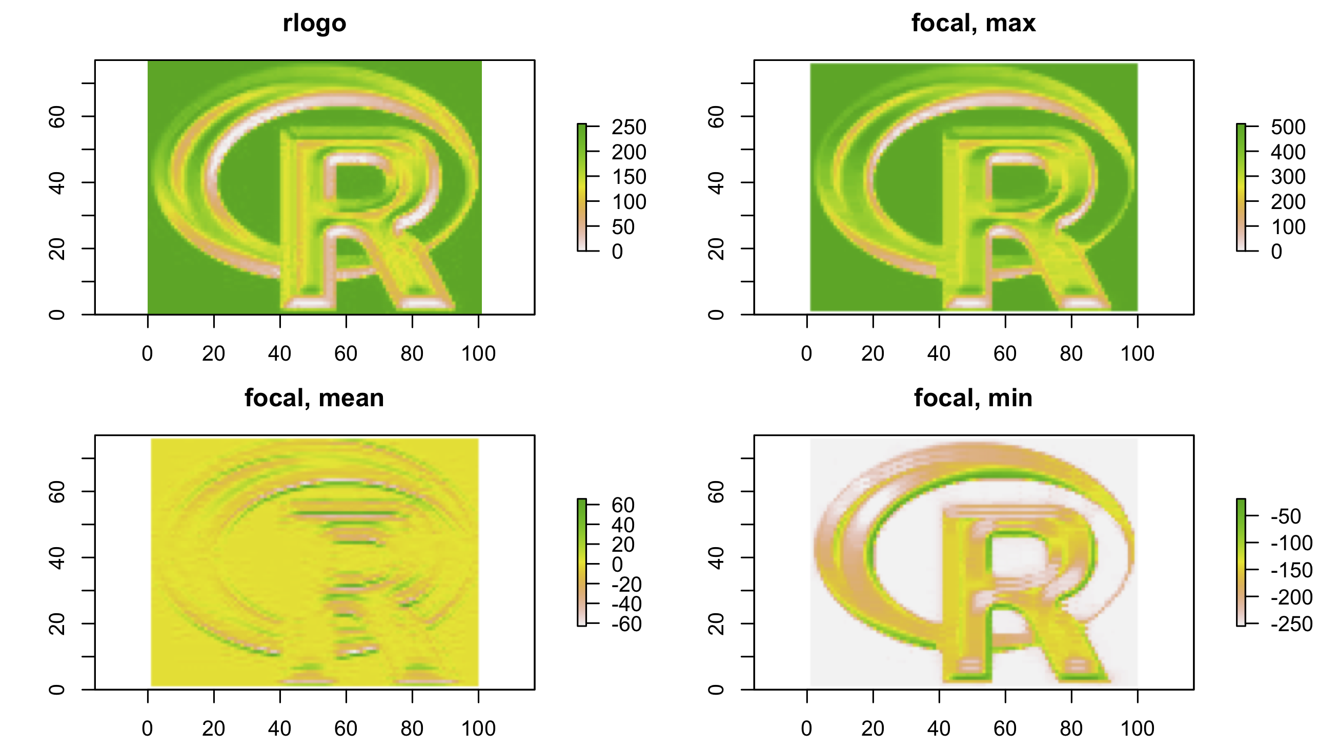
Apply a line detection filter to raster(system.file("external/rlogo.grd", package = "raster")) . Plot the result. Hint: Read ?raster::focal() .
r1 <- raster(system.file("external/rlogo.grd", package = "raster"))
# for example: a horizontal line detection
filter <- matrix(c(-1, 2, -1, -1, 2, -1, -1, 2, -1), nrow =3)
filter
#      [,1] [,2] [,3]
# [1,]   -1   -1   -1
# [2,]    2    2    2
# [3,]   -1   -1   -1
rf1 <- focal(r1, w = filter, fun = max)
rf2 <- focal(r1, w = filter, fun = mean)
rf3 <- focal(r1, w = filter, fun = min)
par(mfrow=c(2,2), mar=c(3,3,3,3))
plot(r1, main = "rlogo")
plot(rf1, main = "focal, max")
plot(rf2, main = "focal, mean")
plot(rf3, main = "focal, min")
Q6
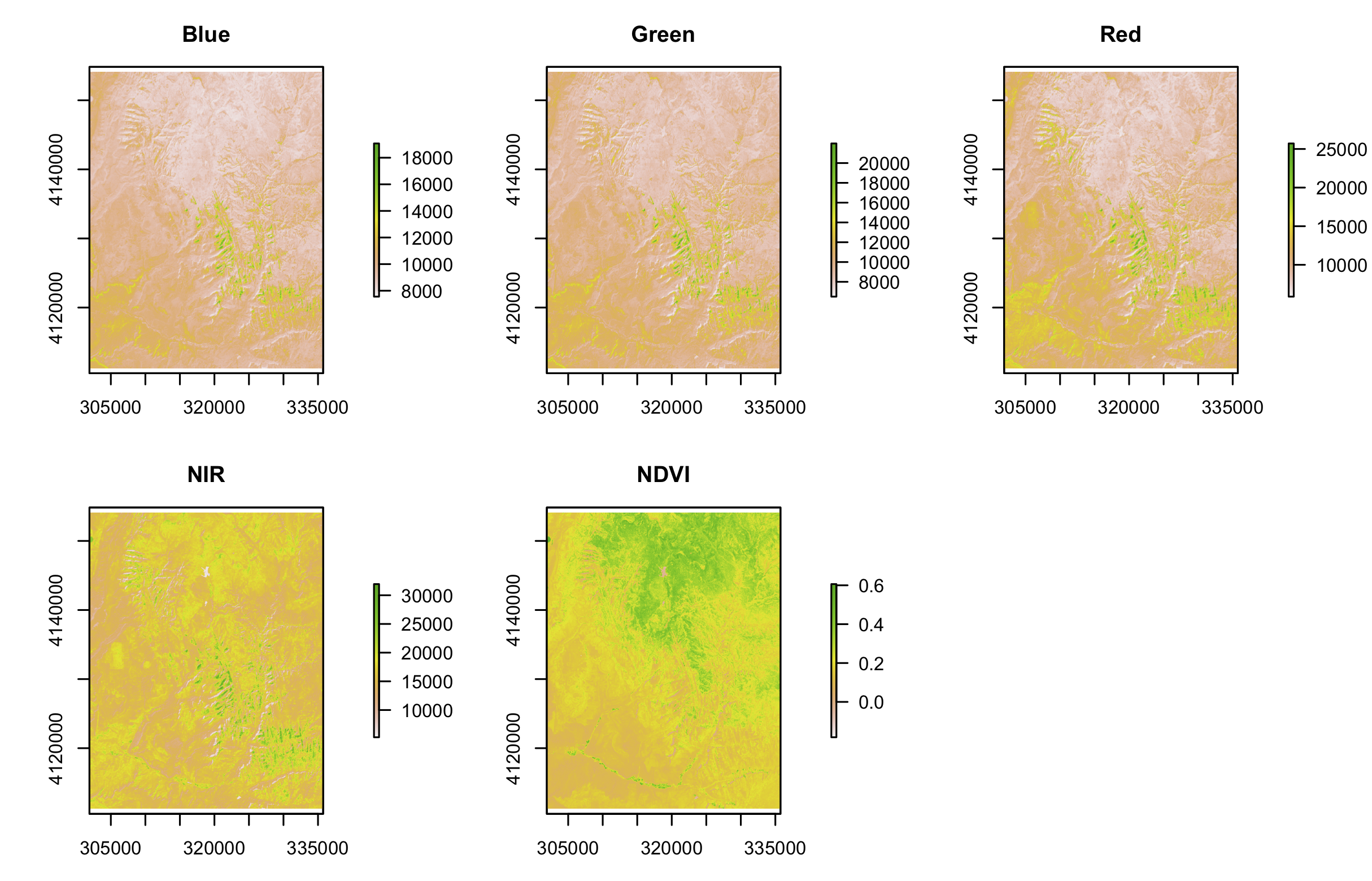
Calculate the NDVI of a Landsat image. Use the Landsat image provided by the spDataLarge package ( system.file("raster/landsat.tif", package="spDataLarge") ).
library(spDaralarge)
landsat_b1 <- raster(system.file("raster/landsat.tif", package="spDataLarge"), band = 1)
landsat_b2 <- raster(system.file("raster/landsat.tif", package="spDataLarge"), band = 2)
landsat_b3 <- raster(system.file("raster/landsat.tif", package="spDataLarge"), band = 3)
landsat_b4 <- raster(system.file("raster/landsat.tif", package="spDataLarge"), band = 4)
# 一般情况下,卫星图的前四个图层分别是Blue、Green、Red、Near Infrared (NIR)
# 所以NDVI的计算只需按照公式 NDVI=(NIR-Red)/(NIR+Red)
NDVI <- (landsat_b4 - landsat_b3)/(landsat_b4 + landsat_b3)
par(mfrow=c(2, 3), mar=c(3, 4, 3, 4))
plot(landsat_b1, main = "Blue")
plot(landsat_b2, main = "Green")
plot(landsat_b3, main = "Red")
plot(landsat_b4, main = "NIR")
plot(NDVI, main = "NDVI")
Q7
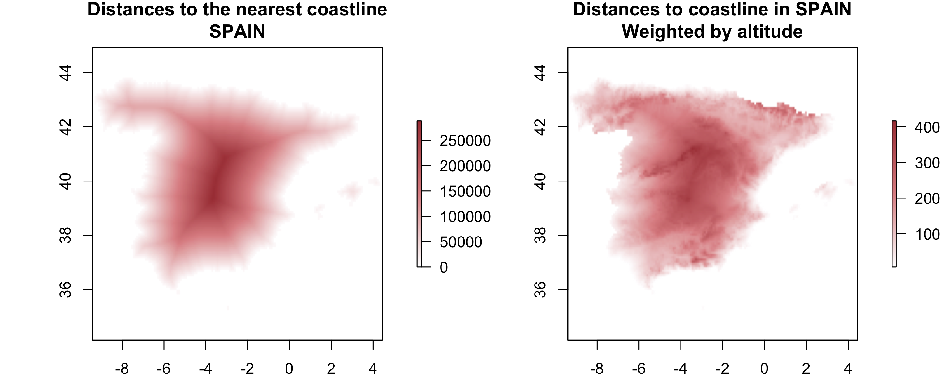
A StackOverflow post shows how to compute distances to the nearest coastline using raster::distance() . Retrieve a digital elevation model of Spain, and compute a raster which represents distances to the coast across the country (hint: use getData() ). Second, use a simple approach to weight the distance raster with elevation (other weighting approaches are possible, include flow direction and steepness); every 100 altitudinal meters should increase the distance to the coast by 10 km. Finally, compute the difference between the raster using the Euclidean distance and the raster weighted by elevation. Note: it may be wise to increase the cell size of the input raster to reduce compute time during this operation.
esp <- getData("alt", country="ESP", mask=TRUE)
# 使用第5章5.3.3中的 aggregate() 函数,降低该栅格分辨率,以免运行时间过长
esp_decrease <- aggregate(esp, fact = 10, fun = mean)
# 由于esp_decrease的最小值是-13,即海拔有低于海平面的负值,因此需要将负值全部视作0
esp_decrease[esp_decrease < 0] = 0
# 将海洋部分的值全部改为 NA
rx <- mask(is.na(esp_decrease), esp_decrease, inverse = TRUE)
# 计算陆地到最近的 NA 的距离,单位是 m
dx <- distance(rx)

# 按照题目要求加权这一距离,即海拔每增加100米,距离海岸线距离增加10 km
dx_weight <- dx + esp_decrease/100 *10000

par(mfrow = c(1,2))
plot(dx, col = colorRampPalette(c("white", "#f07d82", "#b12831"))(256), main = "Distances to the nearest coastline\nSPAIN")
plot(dx_weight, col = colorRampPalette(c("white", "#f07d82", "#b12831"))(256), main = "Distances to coastline in SPAIN\nWeighted by altitude")
原书习题答案详见Chapter 4: Spatial operations。