The exercise solutions of Chapter 3 could be accessed at Chapter 3: Attribute operations. Here I put exercise solutions of my own and explain in Chinese. Maybe these are alterative answers.
第三章 Attribute data operations介绍的是地理数据模型矢量(sf对象)和栅格(raster对象)中,除了地理数据之外(代表空间信息)的其他数据,即非空间的attribute数据。详见书中内容。
解决问题
-
抽取非空间数据的列(Q1)。
-
根据列表名称,抽取满足条件的非空间数据(Q2)。
-
根据列中的变量条件,抽取复合条件的给空间数据(Q3)。
-
抽取某一列后,对其进行统计(Q4)。
-
根据不同变量条件,进行数据的整合统计(Q5,Q6)。
-
将拥有相同列变量的两个矢量对象合并,并能比较这两个对象的差异(Q7,Q8)。
-
会使用变量进行计算,以产生新的变量(Q9,Q10)。
-
更改非空间数据的变量名(Q11,Q12)。
-
综合上述的操作,计算复杂的问题(Q12,Q13)
-
定义新栅格对象,并按条件抽取栅格值(Q14)。
-
能对栅格对象的属性、数据等进行了解(Q15,Q16,Q17)。
所需R包
library(spData)
library(rlang)
library(sf)
library(raster)
library(dplyr)
library(stringr)
library(RQGIS)
data(us_states)
data(us_states_df)
Q1
Create a new object called us_states_name that contains only the NAME column from the us_states object. What is the class of the new object and what makes it geographic?
us_states
# Simple feature collection with 49 features and 6 fields
# geometry type:  MULTIPOLYGON
# dimension:      XY
# bbox:           xmin: -124.7042 ymin: 24.55868 xmax: -66.9824 ymax: 49.38436
# epsg (SRID):    4269
# proj4string:    +proj=longlat +datum=NAD83 +no_defs
# First 10 features:
#    GEOID        NAME   REGION             AREA total_pop_10 total_pop_15
# 1     01     Alabama    South 133709.27 [km^2]      4712651      4830620
# 2     04     Arizona     West 295281.25 [km^2]      6246816      6641928
# 3     08    Colorado     West 269573.06 [km^2]      4887061      5278906
# 4     09 Connecticut Norteast  12976.59 [km^2]      3545837      3593222
# 5     12     Florida    South 151052.01 [km^2]     18511620     19645772
# 6     13     Georgia    South 152725.21 [km^2]      9468815     10006693
# 7     16       Idaho     West 216512.66 [km^2]      1526797      1616547
# 8     18     Indiana  Midwest  93648.40 [km^2]      6417398      6568645
# 9     20      Kansas  Midwest 213037.08 [km^2]      2809329      2892987
# 10    22   Louisiana    South 122345.76 [km^2]      4429940      4625253
#                          geometry
# 1  MULTIPOLYGON (((-88.20006 3...
# 2  MULTIPOLYGON (((-114.7196 3...
# 3  MULTIPOLYGON (((-109.0501 4...
# 4  MULTIPOLYGON (((-73.48731 4...
# 5  MULTIPOLYGON (((-81.81169 2...
# 6  MULTIPOLYGON (((-85.60516 3...
# 7  MULTIPOLYGON (((-116.916 45...
# 8  MULTIPOLYGON (((-87.52404 4...
# 9  MULTIPOLYGON (((-102.0517 4...
# 10 MULTIPOLYGON (((-92.01783 2...
# 三种抽出 NAME 的方式
us_states_names <- us_states[["NAME"]]
us_states_names1 <- us_states$NAME
us_states_names2 <- dplyr::select(us_states, NAME)
Q2
Select columns from the us_states object which contain population data. Obtain the same result using a different command (bonus: try to find three ways of obtaining the same result). Hint: try to use helper functions, such as contains or starts_with from dplyr (see ?contains).
# 直接列出所有含 pop 的列
us_states_pop1 <- dplyr::select(us_states, c("total_pop_10","total_pop_15")) %>% st_drop_geometry()
# 注意,这里不能用 filter(),因为该函数选择满足某条件的行
# 用 contain 找名称包含 pop 的列
popname2 <- names(us_states) %>% vars_select(contains("pop"))
us_states_pop2 <- dplyr::select(us_states, popname2) %>% st_drop_geometry()
# 用 starts_with 找名称开头为 total_pop 的列
popname3 <- names(us_states) %>% vars_select(starts_with("total_pop"))
us_states_pop3 <- data.frame(us_states$total_pop_10, us_states$total_pop_15) %>% set_names(c(popname3))
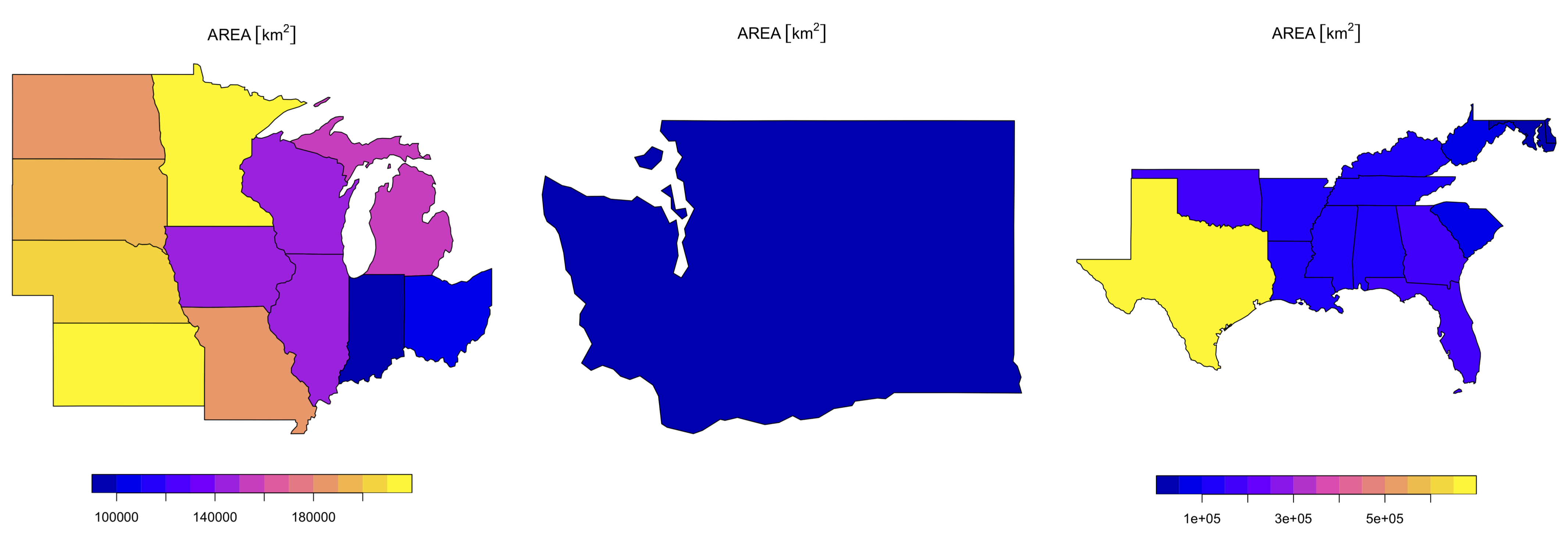
Q3
Find all states with the following characteristics (bonus find and plot them):
-
Belong to the Midwest region.
-
Belong to the West region, have an area below 250,000 km2 and in 2015 a population greater than 5,000,000 residents (hint: you may need to use the function units::set_units() or as.numeric()).
-
Belong to the South region, had an area larger than 150,000 km2 or a total population in 2015 larger than 7,000,000 residents.
# 这时使用了 filter() 函数
midwest <- us_states %>% filter(REGION == "Midwest")
plot(midwest["AREA"]) # 左图

# 由于 AREA 含有单位,必须用 as.numeric() 抽出数字
# 也可以用 units::set_units(),参见原书答案
west.reg <- us_states %>%
  filter(REGION == "West") %>%
  filter(as.numeric(AREA) < 250000) %>%
  filter(total_pop_15 > 5000000)
plot(west.reg["AREA"]) # 中图

# filter() 中可使用各种逻辑符号,这里 "|" 为“或”
south.reg <- us_states %>%
  filter(REGION == "South") %>%
  filter(as.numeric(AREA) > 150000 | total_pop_15 < 7000000)
plot(south.reg["AREA"])  # 右图
Q4
What was the total population in 2015 in the us_states dataset? What was the minimum and maximum total population in 2015?
# 先把 total_pop_15 选出来,再用 summarize() 函数中的各参数计算
total2015 <- dplyr::select(us_states, total_pop_15) %>%
  summarize(pop2015 = sum(total_pop_15, na.rm=TRUE), minpop2015=min(total_pop_15), maxpop2015=max(total_pop_15))
total2015
# Simple feature collection with 1 feature and 3 fields
# geometry type:  MULTIPOLYGON
# dimension:      XY
# bbox:           xmin: -124.7042 ymin: 24.55868 xmax: -66.9824 ymax: 49.38436
# epsg (SRID):    4269
# proj4string:    +proj=longlat +datum=NAD83 +no_defs
#     pop2015 minpop2015 maxpop2015                       geometry
# 1 314375347     579679   38421464 MULTIPOLYGON (((-81.81169 2...
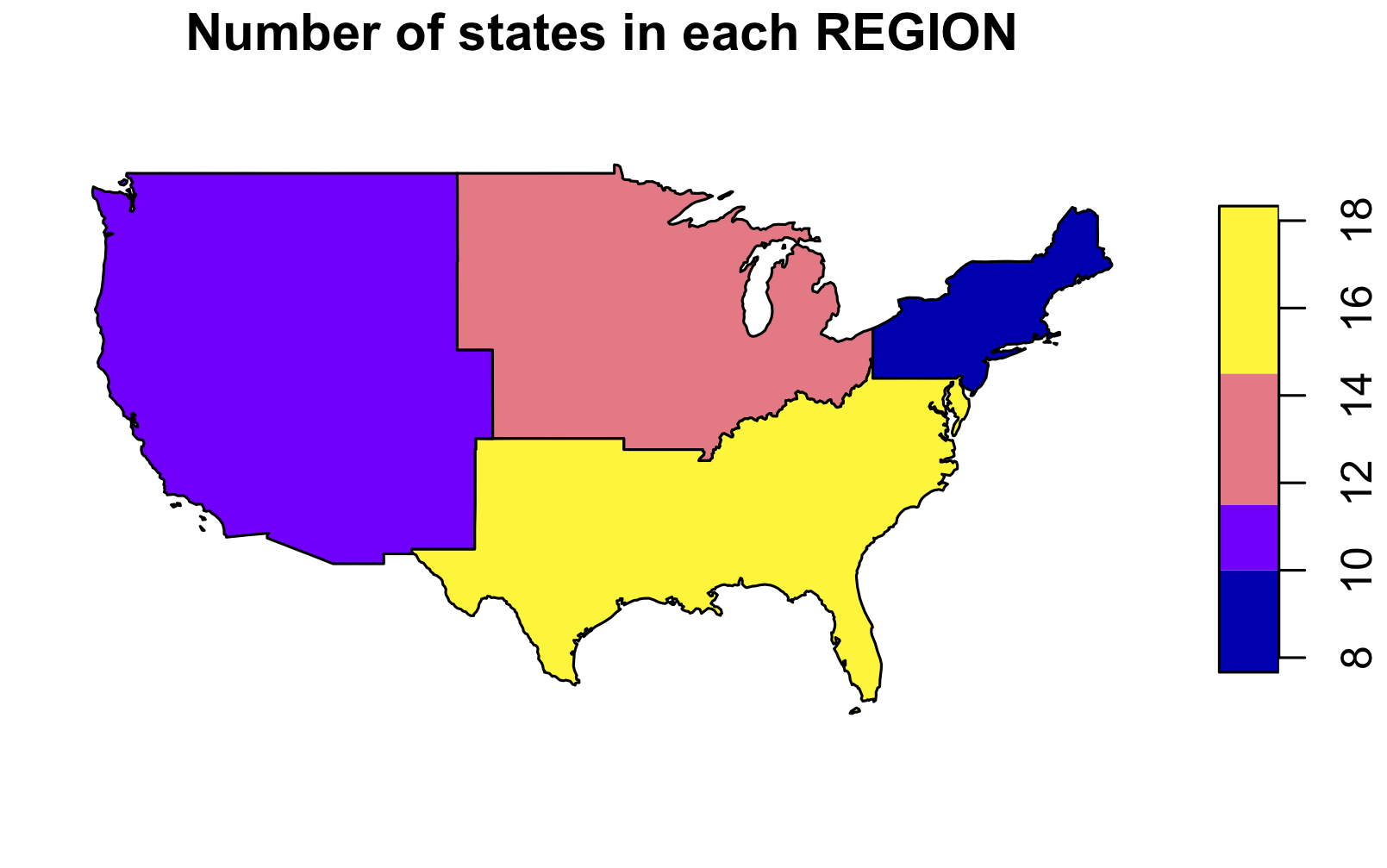
Q5
How many states are there in each region?
# 先把属于各个 REGION 的国家合并起来,再用 summarize() 计算个数
state.region <- group_by(us_states, REGION) %>%
  summarize(number_state = n())
state.region %>% st_drop_geometry()
# # A tibble: 4 x 2
#   REGION   number_state
# * <fct>     <int>
# 1 Norteast      9
# 2 Midwest      12
# 3 South        17
# 4 West         11
plot(state.region["number_state"], main = "Number of states in each REGION")
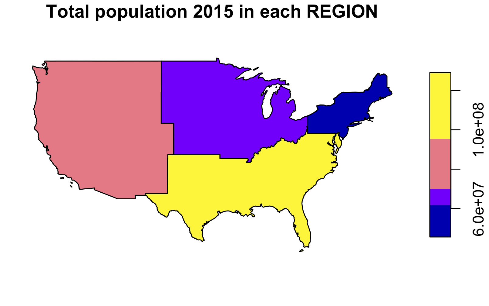
Q6
What was the minimum and maximum total population in 2015 in each region? What was the total population in 2015 in each region?
# 还是先把 REGION 聚集起来,再用 summarize() 计算各个值
pop.region <- group_by(us_states, REGION) %>%
  summarize(pop2015 = sum(total_pop_15, na.rm=TRUE), ncount=n(), maxpop=max(total_pop_15), minpop=min(total_pop_15))
pop.region %>% st_drop_geometry()
# # A tibble: 4 x 5
#   REGION     pop2015 ncount   maxpop minpop
# * <fct>        <dbl>  <int>    <dbl>  <dbl>
# 1 Norteast  55989520      9 19673174 626604
# 2 Midwest   67546398     12 12873761 721640
# 3 South    118575377     17 26538614 647484
# 4 West      72264052     11 38421464 579679
plot(pop.region["pop2015"], main = "Total population 2015 in each REGION")
Q7
Add variables from us_states_df to us_states, and create a new object called us_states_stats. What function did you use and why? Which variable is the key in both datasets? What is the class of the new object?
us_states_df
# # A tibble: 51 x 5
#    state median_income_10 median_income_15 poverty_level_10 poverty_level_15
#    <chr>            <dbl>            <dbl>            <dbl>            <dbl>
#  1 Alab…            21746            22890           786544           887260
#  2 Alas…            29509            31455            64245            72957
#  3 Ariz…            26412            26156           933113          1180690
#  4 Arka…            20881            22205           502684           553644
#  5 Cali…            27207            27035          4919945          6135142
#  6 Colo…            29365            30752           584184           653969
#  7 Conn…            32258            33226           314306           366351
#  8 Dela…            29205            30329            93857           108315
#  9 Dist…            35264            40884           101767           110365
# 10 Flor…            24812            24654          2502365          3180109
# # … with 41 more rows
# us_states_df 与us_states 有一列名称相同,根据这一同名称的列,合并两数据
us_states_stats <- left_join(us_states, us_states_df, by = c(NAME = "state"))
Q8
us_states_df has two more rows than us_states. How can you find them? (hint: try to use the dplyr::anti_join() function)
# 若setdiff()函数内对象的顺序不同,则结果不同。其意义是:根据第二个对象,对比第一个对象。
setdiff(us_states$NAME, us_states_df$state)
# character(0)
setdiff(us_states_df$state, us_states$NAME)
# [1] "Alaska" "Hawaii"
# 即第一个对象跟第二个对象相比,多出了"Alaska" "Hawaii"
Q8.result <- anti_join(us_states_df, us_states, by = c(state = "NAME"))
Q8.result
# # A tibble: 2 x 5
#   state  median_income_10 median_income_15 poverty_level_10 poverty_level_15
#   <chr>             <dbl>            <dbl>            <dbl>            <dbl>
# 1 Alaska            29509            31455            64245            72957
# 2 Hawaii            29945            31051           124627           153944
Q9
What was the population density in 2015 in each state? What was the population density in 2010 in each state?
# 人口密度即人口总数除以面积
# 这样的非空间属性数据的计算,用 mutate() 函数,得出一个新变量
density <- us_states %>%
  mutate(density2015 = total_pop_15 / as.numeric(AREA), density2010 = total_pop_10 / as.numeric(AREA))
# 只列出新生成的人口密度这一列
head(density$density2015)
# [1]  36.12779  22.49356  19.58247 276.90036 130.05966  65.52090
head(density$density2010)
# [1]  35.24551  21.15548  18.12889 273.24879 122.55130  61.99903
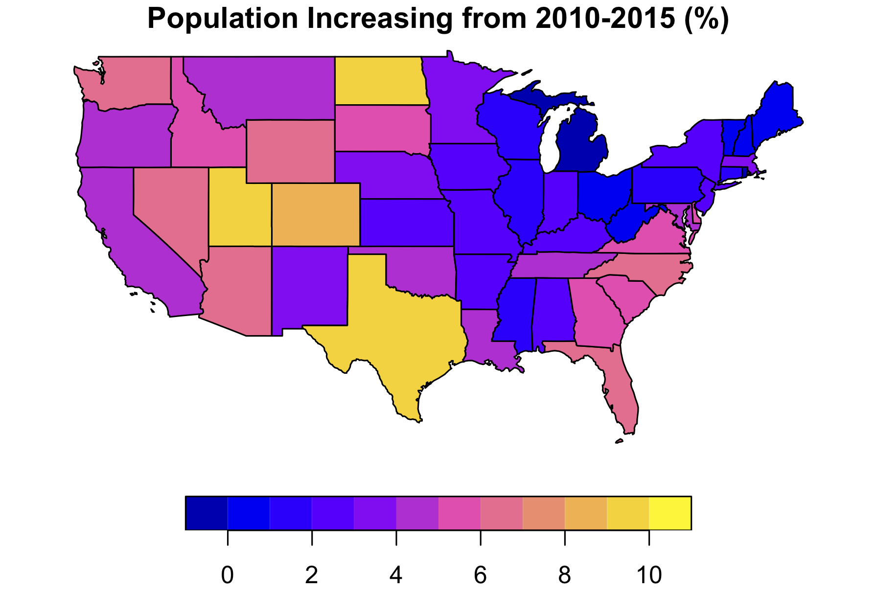
Q10
How much has population density changed between 2010 and 2015 in each state? Calculate the change in percentages and map them.
# 要求人口增长百分比,因此要乘以100
percentage <- density %>%
  mutate(increase.percentage = 100 * (density$density2015 - density$density2010) / density$density2010)
plot(percentage["increase.percentage"], main = "Percentage of Population Increasing from 2010-2015")
Q11
Change the columns’ names in us_states to lowercase. (Hint: helper functions - tolower() and colnames() may help.)
new <- c("Geoid", "Name", "Region", "Aera", "Total_pop_15", "Total_pop_10", "geometry")
# 用 set_names() 函数重命名,必须也包含 geometry 列,否则运行出错
us_states %>% set_names(new)
原书答案使用了提示中的函数,更简单。
Q12
Using us_states and us_states_df create a new object called us_states_sel. The new object should have only two variables - median_income_15 and geometry. Change the name of the median_income_15 column to Income.
# 选出某一列,使用 dplyr::select()函数
# 这个函数自动将空间数据 geometry 附带选出,即输出的仍是包含空间数据的 sf 对象
us_states_sel <- left_join(us_states, us_states_df, by = c(NAME = "state")) %>%
  dplyr::select(median_income_15)
us_states_sel
# Simple feature collection with 49 features and 1 field
# geometry type:  MULTIPOLYGON
# dimension:      XY
# bbox:           xmin: -124.7042 ymin: 24.55868 xmax: -66.9824 ymax: 49.38436
# epsg (SRID):    4269
# proj4string:    +proj=longlat +datum=NAD83 +no_defs
# First 10 features:
#    median_income_15                       geometry
# 1             22890 MULTIPOLYGON (((-88.20006 3...
# 2             26156 MULTIPOLYGON (((-114.7196 3...
# 3             30752 MULTIPOLYGON (((-109.0501 4...
# 4             33226 MULTIPOLYGON (((-73.48731 4...
# 5             24654 MULTIPOLYGON (((-81.81169 2...
# 6             25588 MULTIPOLYGON (((-85.60516 3...
# 7             23558 MULTIPOLYGON (((-116.916 45...
# 8             25834 MULTIPOLYGON (((-87.52404 4...
# 9             27315 MULTIPOLYGON (((-102.0517 4...
# 10            24014 MULTIPOLYGON (((-92.01783 2...

# 改变量名,用新定义的 Income 替换原来的 "median_income_15"
sel_rn <- rename(us_states_sel, Income = "median_income_15")
names(sel_rn)
# [1] "Income"   "geometry"
Q13
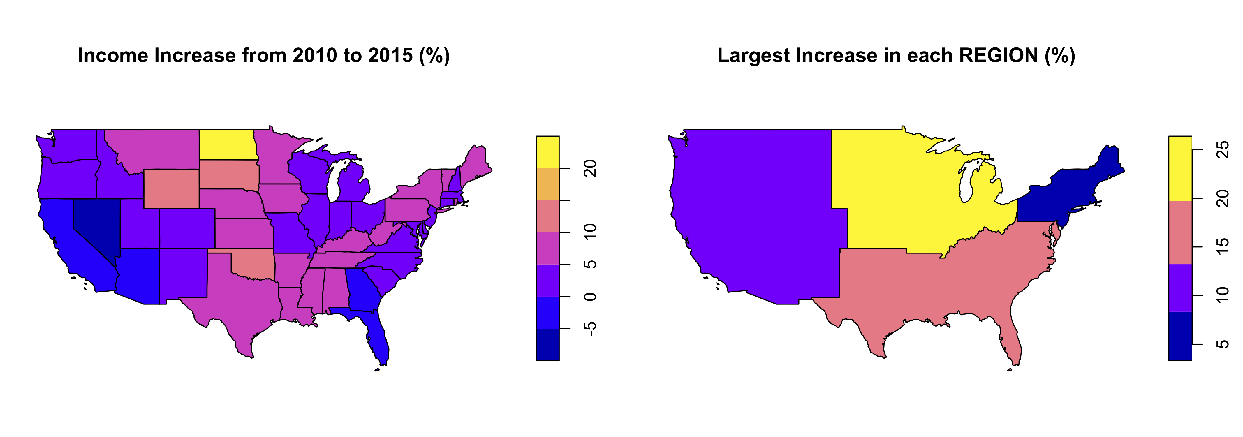
Calculate the change in median income between 2010 and 2015 for each state. Bonus: What was the minimum, average and maximum median income in 2015 for each region? What is the region with the largest increase of the median income?
# Q12 中合并的 us_states_sel 只选择了2015年的数据,因此需要重新合并
us_states_comb <- left_join(us_states, us_states_df, by = c(NAME = "state"))
us_income_inc_per <- mutate(us_states_comb, income.increase.per = 100 * (median_income_15 - median_income_10) / median_income_10)
us_income_inc_per["income.increase.per"]
plot(us_income_inc_per["income.increase.per"], main = "Income Increase from 2010 to 2015 (%)")
# 左图

# 再次用 group_by() 和 summarize() 结合法,输出统计值
Q13_result2 <- us_income_inc_per %>%
  group_by(REGION) %>%
  summarize(min.income2015 = min(median_income_15), mean.income2015 = mean(median_income_15), max.income2015 = max(median_income_15), largest_income = max(income.increase.per))
Q13_result2 %>% st_drop_geometry()
# # A tibble: 4 x 5
#   REGION   min.income2015 mean.income2015 max.income2015 largest_income
# * <fct>             <dbl>           <dbl>          <dbl>          <dbl>
# 1 Norteast          25284          29712.          33226           6.19
# 2 Midwest           25308          27493.          31014          23.5
# 3 South             21438          26369.          40884          15.9
# 4 West              23428          26763.          30752          10.5
plot(Q13_result2["largest_income"], main = "Largest Increase in each REGION (%)")
# 右图
Q14
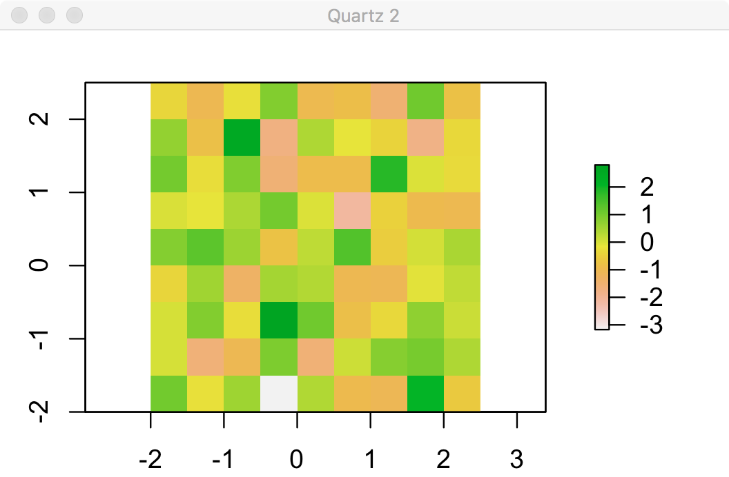
Create a raster from scratch with nine rows and columns and a resolution of 0.5 decimal degrees (WGS84). Fill it with random numbers. Extract the values of the four corner cells.
# 随机值选取,使用rnorm() 函数
# 行数、列数、分辨率都定义过的时候,该栅格的x、y的长度范围必须等于 行数×分辨率、列数×分辨率
set.seed(0627)
raster1 <- raster(ncols=9, nrows=9, res=0.5, xmn = -2, xmx = 2.5, ymn = -2, ymx = 2.5, vals=rnorm(81))
raster1[c(1,9,73,81)] # 最机械的方法,把四个角的cell号码找出来,输出其值
# [1] -0.3643698 -0.7979036  1.0453157 -0.6185311
# 或者
raster1[1,1]
# [1] -0.3643698
raster1[1,9]
# [1] -0.7979036
raster1[9,1]
# [1] 1.045316
raster1[9,9]
# [1] -0.6185311
Q15
What is the most common class of our example raster grain (hint: modal() )?
# grain 是一个分类栅格,modal() 可查看其属性
modal(grain)
# class      : RasterLayer
# dimensions : 6, 6, 36  (nrow, ncol, ncell)
# resolution : 0.5, 0.5  (x, y)
# extent     : -1.5, 1.5, -1.5, 1.5  (xmin, xmax, ymin, ymax)
# crs        : +proj=longlat +datum=WGS84 +ellps=WGS84 +towgs84=0,0,0
# source     : memory
# names      : layer
# values     : 1, 3  (min, max)
# attributes :
#  ID VALUE
#   1  clay
#   2  silt
#   3  sand
Q16
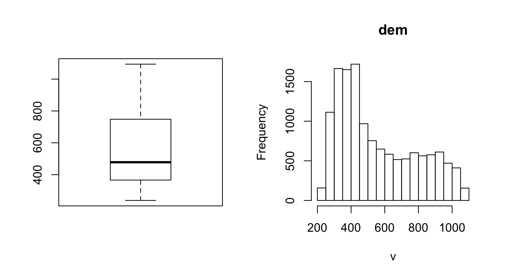
Plot the histogram and the boxplot of the data(dem, package = "RQGIS") raster.
library(RQGIS)
class(dem)
par(mfrow = c(1,2))
boxplot(dem)
hist(dem)
Q17
原本书中并没有第17题,而习题答案中却有第17题,因此也在此附上。
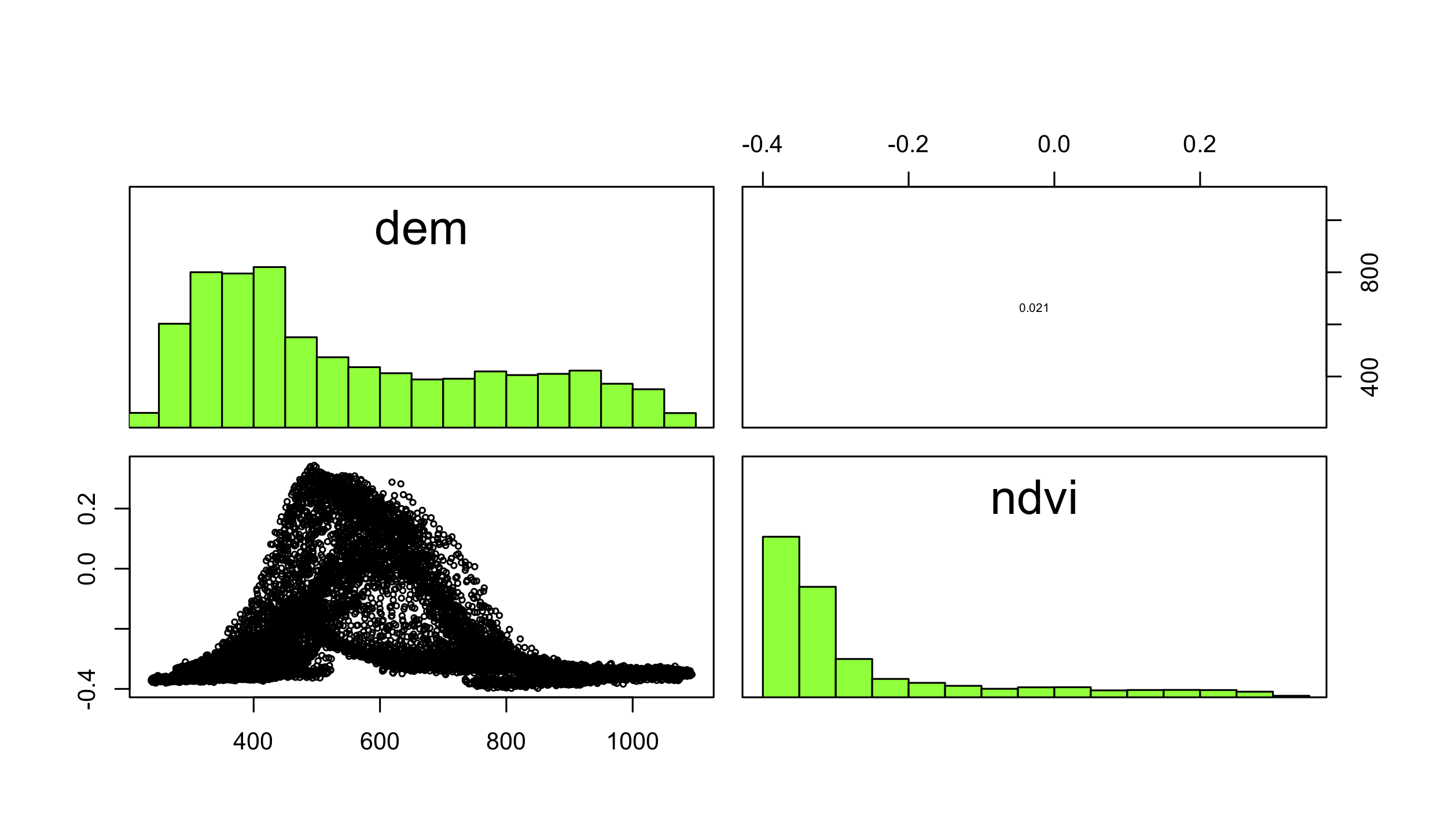
Now attach also data(ndvi, package = "RQGIS"). Create a raster stack using dem and ndvi, and make a pairs() plot.
data(ndvi, package = "RQGIS")
s = stack(dem, ndvi)
pairs(s)
若要查看原书中的详细答案,请参阅Chapter 3: Attribute operations.