Geocomputation with R is a great book on geographic data analysis, visualization and modeling. This book is open source. This makes it accessible for every one. I read this book and learned a lot. If the authors allow it, I even want to translate it into Chinese and let more Chinese researchers learn from it. But at first, I want to share my learning from this book by giving my own answers to exercises in each chapter.
Actually you can find the solutions written by the author Exercises and solutions. Here I did it myself and translated into Chinese.
第二章Geographic data in R 主要讲解两种基本的地理数据模型:矢量和栅格。详见书中内容。
解决问题
-
如何查看一个矢量或栅格对象的各项信息和属性值(Q1)。
-
如何在地图上输出对应的非空间数据(Q2)。
-
如何从矢量对象(全局地图)中取亚集(某部分地图),并输出其在整体背景下的地图(Q3)。
-
会定义一个自定义栅格对象(Q4)。
-
会从数据包中提取栅格数据(Q5)。
所需R包
library(sf)          # classes and functions for vector data
library(raster)      # classes and functions for raster data
library(spData)        # load geographic data
library(spDataLarge)   # load larger geographic data
Q1
Use summary() on the geometry column of the world data object. What does the output tell us about:
- Its geometry type?
- The number of countries?
- Its coordinate reference system (CRS)?
summary(world)
world
从summary(world)结果中的geom列得知:几何类型(geometry type)是MULTIPOLYGON即复合多边形;共有177个国家的数据;坐标参考系(CRS)在这一结果中没有显示完全,world直接输出则可完全显示+proj=longlat +datum=WGS84 +no_defs 或 epsg:4326(关于坐标参考系请阅读Chapter 6 Projecting geographic data)。
Q2
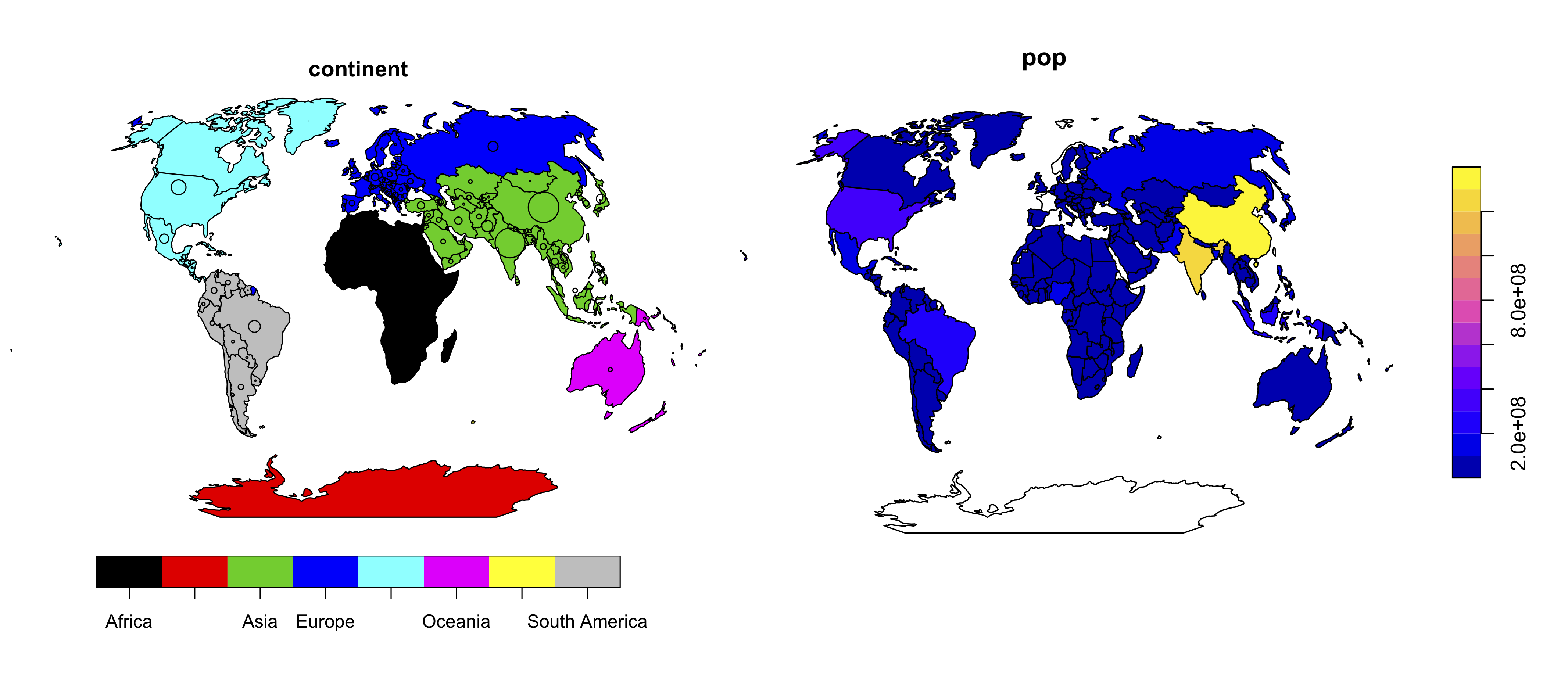
Run the code that ‘generated’ the map of the world in Figure 2.5 at the end of Section 2.2.4. Find two similarities and two differences between the image on your computer and that in the book.
- What does the
cexargument do (see?plot)? - Why was
cexset to thesqrt(world$pop) / 10000? - Bonus: experiment with different ways to visualize the global population.
plot(world["continent"], reset = FALSE)
# reset = FALSE 表示返回结果后地图元素还能继续用于下一步,此处即计算cex的大小
cex = sqrt(world$pop) / 10000
world_cents = st_centroid(world, of_largest = TRUE)
# of_largest = TRUE 表示输出最大的多边形的中心,本例中即整个国家的中心,而不是国家里各个小的省份
plot(st_geometry(world_cents), add = TRUE, cex = cex)

生成的地图中,数据、颜色都与书中相似,而投影、多边形形状、标签却不同。cex 参数定义中心的图标大小,如果不将人口数开平方根再除以1000,图标将太大了。另外,还有好几种其他方法输出全世界的人口分布:
# 根据第6章,改变投影
world_wintri = lwgeom::st_transform_proj(world, crs = "+proj=wintri")
plot(world_wintri["continent"], reset = FALSE, pal = c(1,2,3,4,5,6,7,8))
cex_wintri = sqrt(world_wintri$pop) / 10000
world_cents_wintri = st_centroid(world_wintri, of_largest = TRUE)
plot(st_geometry(world_cents_wintri), add = TRUE, cex = cex_wintri)
# 直接输出pop数据
plot(world_wintri["pop"])
Q3
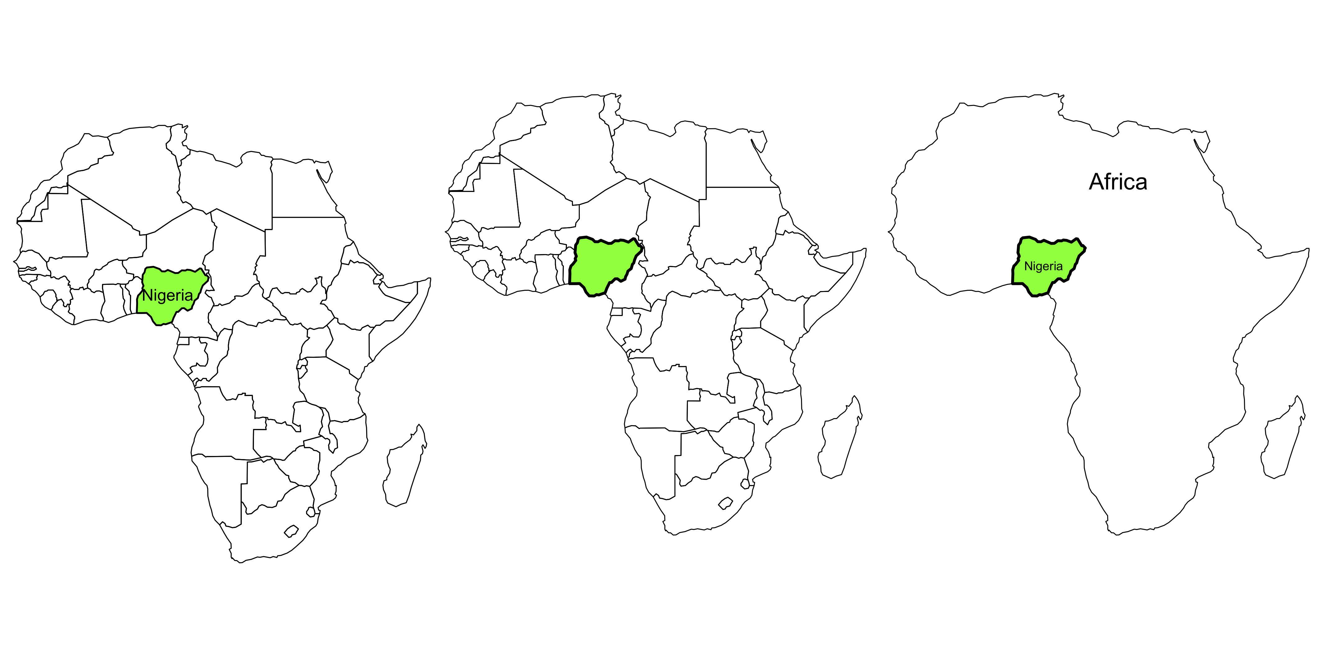
Use plot() to create maps of Nigeria in context (see Section 2.2.4). Adjust the lwd, col and expandBB arguments of plot(). Challenge: read the documentation of text() and annotate the map.
world_africa <- world[world$continent == "Africa", ]
nigeria <- world[world$name_long == "Nigeria",]
# 注意不要忘记了后面的逗号
# Left graph
plot(st_geometry(nigeria), expandBB = c(4, 2, 3, 4), col = "green", lwd = 1.8)
plot(st_geometry(world_africa), add = TRUE)
text(7.8, 9, labels = "Nigeria")
# Middle graph
plot(st_geometry(world_africa))
plot(st_geometry(nigeria), col = "green", lwd = 3, add = TRUE)
# Right graph
africa <- st_union(world_africa)
plot(st_geometry(africa))
plot(st_geometry(nigeria), col = "green", lwd = 3, add = TRUE)
text(x = c(7.8, 20), y = c(9, 23), labels = c("Nigeria", "Africa"), cex=c(0.8,1.5))
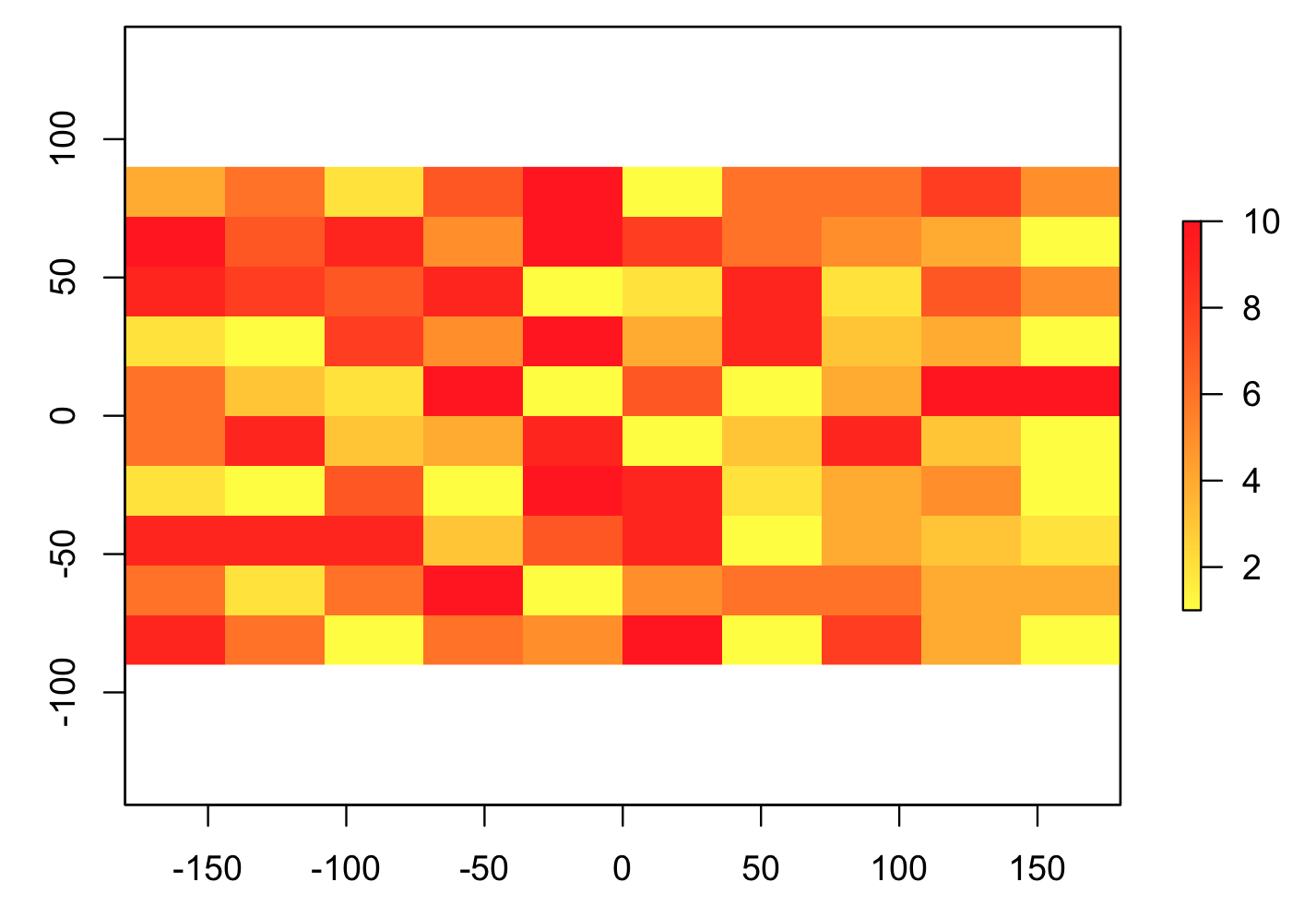
Q4
Create an empty RasterLayer object called my_raster with 10 columns and 10 rows. Assign random values between 0 and 10 to the new raster and plot it.
my_raster <- raster(nrows = 10, ncols = 10, vals = sample(1:10, size = 100, replace = TRUE))
palette <- colorRampPalette(c("yellow", "red"))(256)
plot(my_raster, col=palette)
Q5
Read-in the raster/nlcd2011.tif file from the spDataLarge package. What kind of information can you get about the properties of this file?
nlcd <- raster(system.file("raster/nlcd2011.tif", package = "spDataLarge"))
nlcd
# class      : RasterLayer
# dimensions : 1359, 1073, 1458207  (nrow, ncol, ncell)
# resolution : 31.5303, 31.52466  (x, y)
# extent     : 301903.3, 335735.4, 4111244, 4154086  (xmin, xmax, ymin, ymax)
# crs        : +proj=utm +zone=12 +ellps=GRS80 +towgs84=0,0,0,0,0,0,0 +units=m +no_defs
# source     : /Library/Frameworks/R.framework/Versions/3.5/Resources/library/spDataLarge/raster/nlcd2011.tif
# names      : nlcd2011
# values     : 11, 95  (min, max)
所有必要信息即可从结果中获得。
原书习题答案参见:Chapter 2: Geographic data in R。